Data wrangling: more on filter() and select()

r-basics
tidyverse
Author

Jessica Cooperstone

Published

August 26, 2024


Artwork by @allison_horst

1 Introduction

We are going to start off this semester of code club with a series of sessions on how to “wrangle” your data. It can be a struggle to get data into a format that is amenable for analysis, so we will be going through a series of functions and approaches that will get you more comfortable with manipulating your data.

“Yet far too much handcrafted work — what data scientists call “data wrangling,” “data munging” and “data janitor work” — is still required. Data scientists, according to interviews and expert estimates, spend from 50 percent to 80 percent of their time mired in this more mundane labor of collecting and preparing unruly digital data, before it can be explored for useful nuggets.” - For Big-Data Scientists, ‘Janitor Work’ Is Key Hurdle to Insights, NY Times

If you don’t have R and RStudio on your computer, you can find instructions for installation here. You can also find some additional introductory material on getting set up in RStudio here.

1.0.1 Poll - who is new to R?

1.1 Load libraries

library(tidyverse)
── Attaching core tidyverse packages ──────────────────────── tidyverse 2.0.0 ──
✔ dplyr     1.1.3     ✔ readr     2.1.4
✔ forcats   1.0.0     ✔ stringr   1.5.1
✔ ggplot2   3.4.4     ✔ tibble    3.2.1
✔ lubridate 1.9.2     ✔ tidyr     1.3.0
✔ purrr     1.0.2     
── Conflicts ────────────────────────────────────────── tidyverse_conflicts() ──
✖ dplyr::filter() masks stats::filter()
✖ dplyr::lag()    masks stats::lag()
ℹ Use the conflicted package (<http://conflicted.r-lib.org/>) to force all conflicts to become errors

1.2 Data

We are going to use data from The World Factbook, put together by the CIA to “provides basic intelligence on the history, people, government, economy, energy, geography, environment, communications, transportation, military, terrorism, and transnational issues for 265 world entities.” I thought this data would give us some opportunities to flex our R skills, and learn a bit about the world.

The data we are going to download can be found here, though I have saved the file, added it to our Code Club Github, and included some code below for you to download it.

download.file(
  url = "https://raw.githubusercontent.com/osu-codeclub/osu-codeclub.github.io/main/posts/S08E01_wrangling_01/data/factbook-2015.csv",
  destfile = "factbook_download_2015.csv"
)

You should now see the file “factbook_download_2015.csv” in your working directory.

We can read it in using the tidyverse function from the readr package called read_csv().

factbook_2015 <- read_csv("factbook_download_2015.csv")
Rows: 217 Columns: 53
── Column specification ────────────────────────────────────────────────────────
Delimiter: ","
chr  (2): Country Name, Country Code
dbl (51): Population, total, Population growth (annual %), Surface area (sq....

ℹ Use `spec()` to retrieve the full column specification for this data.
ℹ Specify the column types or set `show_col_types = FALSE` to quiet this message.

Let’s get a better handle on this data. We can use the function glimpse() to get a “glimpse” at our data.

glimpse(factbook_2015)
Rows: 217
Columns: 53
$ `Country Name`                                                                                     <chr> …
$ `Country Code`                                                                                     <chr> …
$ `Population, total`                                                                                <dbl> …
$ `Population growth (annual %)`                                                                     <dbl> …
$ `Surface area (sq. km)`                                                                            <dbl> …
$ `Poverty headcount ratio at national poverty lines (% of population)`                              <dbl> …
$ `GNI, Atlas method (current US$)`                                                                  <dbl> …
$ `GNI per capita, Atlas method (current US$)`                                                       <dbl> …
$ `GNI, PPP (current international $)`                                                               <dbl> …
$ `GNI per capita, PPP (current international $)`                                                    <dbl> …
$ `Income share held by lowest 20%`                                                                  <dbl> …
$ `Life expectancy at birth, total (years)`                                                          <dbl> …
$ `Fertility rate, total (births per woman)`                                                         <dbl> …
$ `Adolescent fertility rate (births per 1,000 women ages 15-19)`                                    <dbl> …
$ `Contraceptive prevalence, any method (% of married women ages 15-49)`                             <dbl> …
$ `Births attended by skilled health staff (% of total)`                                             <dbl> …
$ `Mortality rate, under-5 (per 1,000 live births)`                                                  <dbl> …
$ `Prevalence of underweight, weight for age (% of children under 5)`                                <dbl> …
$ `Immunization, measles (% of children ages 12-23 months)`                                          <dbl> …
$ `Primary completion rate, total (% of relevant age group)`                                         <dbl> …
$ `School enrollment, secondary (% gross)`                                                           <dbl> …
$ `School enrollment, primary and secondary (gross), gender parity index (GPI)`                      <dbl> …
$ `Prevalence of HIV, total (% of population ages 15-49)`                                            <dbl> …
$ `Forest area (sq. km)`                                                                             <dbl> …
$ `Water productivity, total (constant 2015 US$ GDP per cubic meter of total freshwater withdrawal)` <dbl> …
$ `Energy use (kg of oil equivalent per capita)`                                                     <dbl> …
$ `CO2 emissions (metric tons per capita)`                                                           <dbl> …
$ `Electric power consumption (kWh per capita)`                                                      <dbl> …
$ `GDP (current US$)`                                                                                <dbl> …
$ `GDP growth (annual %)`                                                                            <dbl> …
$ `Inflation, GDP deflator (annual %)`                                                               <dbl> …
$ `Agriculture, forestry, and fishing, value added (% of GDP)`                                       <dbl> …
$ `Industry (including construction), value added (% of GDP)`                                        <dbl> …
$ `Exports of goods and services (% of GDP)`                                                         <dbl> …
$ `Imports of goods and services (% of GDP)`                                                         <dbl> …
$ `Gross capital formation (% of GDP)`                                                               <dbl> …
$ `Revenue, excluding grants (% of GDP)`                                                             <dbl> …
$ `Start-up procedures to register a business (number)`                                              <dbl> …
$ `Market capitalization of listed domestic companies (% of GDP)`                                    <dbl> …
$ `Military expenditure (% of GDP)`                                                                  <dbl> …
$ `Mobile cellular subscriptions (per 100 people)`                                                   <dbl> …
$ `High-technology exports (% of manufactured exports)`                                              <dbl> …
$ `Merchandise trade (% of GDP)`                                                                     <dbl> …
$ `Net barter terms of trade index (2015 = 100)`                                                     <dbl> …
$ `External debt stocks, total (DOD, current US$)`                                                   <dbl> …
$ `Total debt service (% of GNI)`                                                                    <dbl> …
$ `Net migration`                                                                                    <dbl> …
$ `Personal remittances, paid (current US$)`                                                         <dbl> …
$ `Foreign direct investment, net inflows (BoP, current US$)`                                        <dbl> …
$ `Net ODA received per capita (current US$)`                                                        <dbl> …
$ `GDP per capita (current US$)`                                                                     <dbl> …
$ `Foreign direct investment, net (BoP, current US$)`                                                <dbl> …
$ `Inflation, consumer prices (annual %)`                                                            <dbl> …

We see that Country Name and Country Code are character columns while the others are numeric (i.e., dbl).

We can look at this data another way, using the function head() to look at the first six rows, and every column.

head(factbook_2015)
# A tibble: 6 × 53
  `Country Name` `Country Code` `Population, total` Population growth (annual …¹
  <chr>          <chr>                        <dbl>                        <dbl>
1 Afghanistan    AFG                       33753499                        3.12 
2 Albania        ALB                        2880703                       -0.291
3 Algeria        DZA                       39543154                        2.00 
4 American Samoa ASM                          51368                       -1.64 
5 Andorra        AND                          71746                        0.174
6 Angola         AGO                       28127721                        3.62 
# ℹ abbreviated name: ¹​`Population growth (annual %)`
# ℹ 49 more variables: `Surface area (sq. km)` <dbl>,
#   `Poverty headcount ratio at national poverty lines (% of population)` <dbl>,
#   `GNI, Atlas method (current US$)` <dbl>,
#   `GNI per capita, Atlas method (current US$)` <dbl>,
#   `GNI, PPP (current international $)` <dbl>,
#   `GNI per capita, PPP (current international $)` <dbl>, …

1.2.1 Cleaning column names

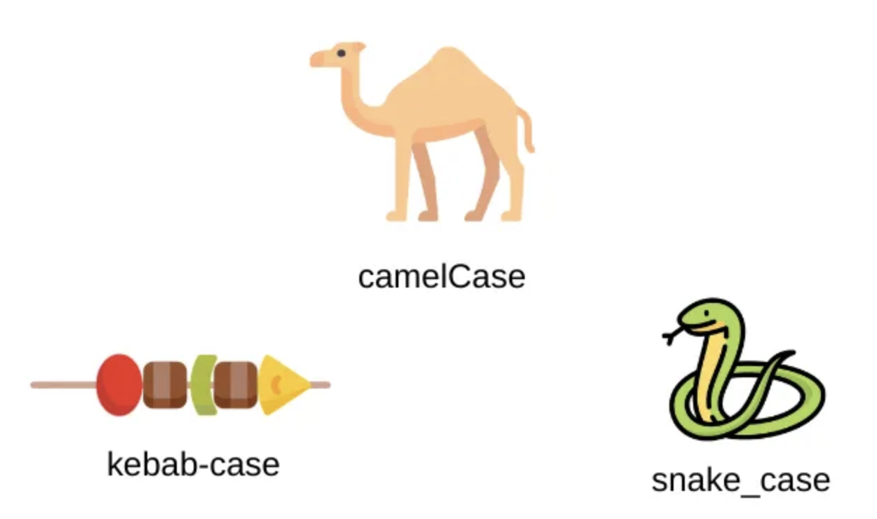
It looks like we have some column names that don’t use standard R practices (i.e., they have spaces, start with numbers). This isn’t a critical problem (meaning you can use column names like this - we know that because we have them here!) but it does make things slightly more difficult. The main difficulty is that you will have to refer to column names surrounded in back ticks and this can be annoying.

factbook_2015$`Country Name`

Let’s use the function clean_names() from the janitor package to clean those names up.

First, install the package janitor if you don’t have it.

install.packages("janitor")

Then we can load the package and clean up our column names.

library(janitor)

Attaching package: 'janitor'
The following objects are masked from 'package:stats':

    chisq.test, fisher.test
# old column names
colnames(factbook_2015)
 [1] "Country Name"                                                                                    
 [2] "Country Code"                                                                                    
 [3] "Population, total"                                                                               
 [4] "Population growth (annual %)"                                                                    
 [5] "Surface area (sq. km)"                                                                           
 [6] "Poverty headcount ratio at national poverty lines (% of population)"                             
 [7] "GNI, Atlas method (current US$)"                                                                 
 [8] "GNI per capita, Atlas method (current US$)"                                                      
 [9] "GNI, PPP (current international $)"                                                              
[10] "GNI per capita, PPP (current international $)"                                                   
[11] "Income share held by lowest 20%"                                                                 
[12] "Life expectancy at birth, total (years)"                                                         
[13] "Fertility rate, total (births per woman)"                                                        
[14] "Adolescent fertility rate (births per 1,000 women ages 15-19)"                                   
[15] "Contraceptive prevalence, any method (% of married women ages 15-49)"                            
[16] "Births attended by skilled health staff (% of total)"                                            
[17] "Mortality rate, under-5 (per 1,000 live births)"                                                 
[18] "Prevalence of underweight, weight for age (% of children under 5)"                               
[19] "Immunization, measles (% of children ages 12-23 months)"                                         
[20] "Primary completion rate, total (% of relevant age group)"                                        
[21] "School enrollment, secondary (% gross)"                                                          
[22] "School enrollment, primary and secondary (gross), gender parity index (GPI)"                     
[23] "Prevalence of HIV, total (% of population ages 15-49)"                                           
[24] "Forest area (sq. km)"                                                                            
[25] "Water productivity, total (constant 2015 US$ GDP per cubic meter of total freshwater withdrawal)"
[26] "Energy use (kg of oil equivalent per capita)"                                                    
[27] "CO2 emissions (metric tons per capita)"                                                          
[28] "Electric power consumption (kWh per capita)"                                                     
[29] "GDP (current US$)"                                                                               
[30] "GDP growth (annual %)"                                                                           
[31] "Inflation, GDP deflator (annual %)"                                                              
[32] "Agriculture, forestry, and fishing, value added (% of GDP)"                                      
[33] "Industry (including construction), value added (% of GDP)"                                       
[34] "Exports of goods and services (% of GDP)"                                                        
[35] "Imports of goods and services (% of GDP)"                                                        
[36] "Gross capital formation (% of GDP)"                                                              
[37] "Revenue, excluding grants (% of GDP)"                                                            
[38] "Start-up procedures to register a business (number)"                                             
[39] "Market capitalization of listed domestic companies (% of GDP)"                                   
[40] "Military expenditure (% of GDP)"                                                                 
[41] "Mobile cellular subscriptions (per 100 people)"                                                  
[42] "High-technology exports (% of manufactured exports)"                                             
[43] "Merchandise trade (% of GDP)"                                                                    
[44] "Net barter terms of trade index (2015 = 100)"                                                    
[45] "External debt stocks, total (DOD, current US$)"                                                  
[46] "Total debt service (% of GNI)"                                                                   
[47] "Net migration"                                                                                   
[48] "Personal remittances, paid (current US$)"                                                        
[49] "Foreign direct investment, net inflows (BoP, current US$)"                                       
[50] "Net ODA received per capita (current US$)"                                                       
[51] "GDP per capita (current US$)"                                                                    
[52] "Foreign direct investment, net (BoP, current US$)"                                               
[53] "Inflation, consumer prices (annual %)"                                                           
# use clean_names and save over the current df factbook_2015
factbook_2015 <- clean_names(factbook_2015)

# new column names
colnames(factbook_2015)
 [1] "country_name"                                                                                
 [2] "country_code"                                                                                
 [3] "population_total"                                                                            
 [4] "population_growth_annual_percent"                                                            
 [5] "surface_area_sq_km"                                                                          
 [6] "poverty_headcount_ratio_at_national_poverty_lines_percent_of_population"                     
 [7] "gni_atlas_method_current_us"                                                                 
 [8] "gni_per_capita_atlas_method_current_us"                                                      
 [9] "gni_ppp_current_international"                                                               
[10] "gni_per_capita_ppp_current_international"                                                    
[11] "income_share_held_by_lowest_20_percent"                                                      
[12] "life_expectancy_at_birth_total_years"                                                        
[13] "fertility_rate_total_births_per_woman"                                                       
[14] "adolescent_fertility_rate_births_per_1_000_women_ages_15_19"                                 
[15] "contraceptive_prevalence_any_method_percent_of_married_women_ages_15_49"                     
[16] "births_attended_by_skilled_health_staff_percent_of_total"                                    
[17] "mortality_rate_under_5_per_1_000_live_births"                                                
[18] "prevalence_of_underweight_weight_for_age_percent_of_children_under_5"                        
[19] "immunization_measles_percent_of_children_ages_12_23_months"                                  
[20] "primary_completion_rate_total_percent_of_relevant_age_group"                                 
[21] "school_enrollment_secondary_percent_gross"                                                   
[22] "school_enrollment_primary_and_secondary_gross_gender_parity_index_gpi"                       
[23] "prevalence_of_hiv_total_percent_of_population_ages_15_49"                                    
[24] "forest_area_sq_km"                                                                           
[25] "water_productivity_total_constant_2015_us_gdp_per_cubic_meter_of_total_freshwater_withdrawal"
[26] "energy_use_kg_of_oil_equivalent_per_capita"                                                  
[27] "co2_emissions_metric_tons_per_capita"                                                        
[28] "electric_power_consumption_k_wh_per_capita"                                                  
[29] "gdp_current_us"                                                                              
[30] "gdp_growth_annual_percent"                                                                   
[31] "inflation_gdp_deflator_annual_percent"                                                       
[32] "agriculture_forestry_and_fishing_value_added_percent_of_gdp"                                 
[33] "industry_including_construction_value_added_percent_of_gdp"                                  
[34] "exports_of_goods_and_services_percent_of_gdp"                                                
[35] "imports_of_goods_and_services_percent_of_gdp"                                                
[36] "gross_capital_formation_percent_of_gdp"                                                      
[37] "revenue_excluding_grants_percent_of_gdp"                                                     
[38] "start_up_procedures_to_register_a_business_number"                                           
[39] "market_capitalization_of_listed_domestic_companies_percent_of_gdp"                           
[40] "military_expenditure_percent_of_gdp"                                                         
[41] "mobile_cellular_subscriptions_per_100_people"                                                
[42] "high_technology_exports_percent_of_manufactured_exports"                                     
[43] "merchandise_trade_percent_of_gdp"                                                            
[44] "net_barter_terms_of_trade_index_2015_100"                                                    
[45] "external_debt_stocks_total_dod_current_us"                                                   
[46] "total_debt_service_percent_of_gni"                                                           
[47] "net_migration"                                                                               
[48] "personal_remittances_paid_current_us"                                                        
[49] "foreign_direct_investment_net_inflows_bo_p_current_us"                                       
[50] "net_oda_received_per_capita_current_us"                                                      
[51] "gdp_per_capita_current_us"                                                                   
[52] "foreign_direct_investment_net_bo_p_current_us"                                               
[53] "inflation_consumer_prices_annual_percent"                                                    

By default, clean_names() converst to “snake_case” (where words are separated by an underscore instead of a space).

Note

Having spaces, starting with numbers, or have unallowable characters (e.g., %, ?, !) is only a problem for column names not for cell contents.

What if we want to see a complete list of our countries? We could run the following code to see that:

factbook_2015$country_name
  [1] "Afghanistan"                    "Albania"                       
  [3] "Algeria"                        "American Samoa"                
  [5] "Andorra"                        "Angola"                        
  [7] "Antigua and Barbuda"            "Argentina"                     
  [9] "Armenia"                        "Aruba"                         
 [11] "Australia"                      "Austria"                       
 [13] "Azerbaijan"                     "Bahamas, The"                  
 [15] "Bahrain"                        "Bangladesh"                    
 [17] "Barbados"                       "Belarus"                       
 [19] "Belgium"                        "Belize"                        
 [21] "Benin"                          "Bermuda"                       
 [23] "Bhutan"                         "Bolivia"                       
 [25] "Bosnia and Herzegovina"         "Botswana"                      
 [27] "Brazil"                         "British Virgin Islands"        
 [29] "Brunei Darussalam"              "Bulgaria"                      
 [31] "Burkina Faso"                   "Burundi"                       
 [33] "Cabo Verde"                     "Cambodia"                      
 [35] "Cameroon"                       "Canada"                        
 [37] "Cayman Islands"                 "Central African Republic"      
 [39] "Chad"                           "Channel Islands"               
 [41] "Chile"                          "China"                         
 [43] "Colombia"                       "Comoros"                       
 [45] "Congo, Dem. Rep."               "Congo, Rep."                   
 [47] "Costa Rica"                     "Cote d'Ivoire"                 
 [49] "Croatia"                        "Cuba"                          
 [51] "Curacao"                        "Cyprus"                        
 [53] "Czechia"                        "Denmark"                       
 [55] "Djibouti"                       "Dominica"                      
 [57] "Dominican Republic"             "Ecuador"                       
 [59] "Egypt, Arab Rep."               "El Salvador"                   
 [61] "Equatorial Guinea"              "Eritrea"                       
 [63] "Estonia"                        "Ethiopia"                      
 [65] "Faroe Islands"                  "Fiji"                          
 [67] "Finland"                        "France"                        
 [69] "French Polynesia"               "Gabon"                         
 [71] "Gambia, The"                    "Georgia"                       
 [73] "Germany"                        "Ghana"                         
 [75] "Gibraltar"                      "Greece"                        
 [77] "Greenland"                      "Grenada"                       
 [79] "Guam"                           "Guatemala"                     
 [81] "Guinea"                         "Guinea-Bissau"                 
 [83] "Guyana"                         "Haiti"                         
 [85] "Honduras"                       "Hong Kong SAR, China"          
 [87] "Hungary"                        "Iceland"                       
 [89] "India"                          "Indonesia"                     
 [91] "Iran, Islamic Rep."             "Iraq"                          
 [93] "Ireland"                        "Isle of Man"                   
 [95] "Israel"                         "Italy"                         
 [97] "Jamaica"                        "Japan"                         
 [99] "Jordan"                         "Kazakhstan"                    
[101] "Kenya"                          "Kiribati"                      
[103] "Korea, Dem. People's Rep."      "Korea, Rep."                   
[105] "Kosovo"                         "Kuwait"                        
[107] "Kyrgyz Republic"                "Lao PDR"                       
[109] "Latvia"                         "Lebanon"                       
[111] "Lesotho"                        "Liberia"                       
[113] "Libya"                          "Liechtenstein"                 
[115] "Lithuania"                      "Luxembourg"                    
[117] "Macao SAR, China"               "North Macedonia"               
[119] "Madagascar"                     "Malawi"                        
[121] "Malaysia"                       "Maldives"                      
[123] "Mali"                           "Malta"                         
[125] "Marshall Islands"               "Mauritania"                    
[127] "Mauritius"                      "Mexico"                        
[129] "Micronesia, Fed. Sts."          "Moldova"                       
[131] "Monaco"                         "Mongolia"                      
[133] "Montenegro"                     "Morocco"                       
[135] "Mozambique"                     "Myanmar"                       
[137] "Namibia"                        "Nauru"                         
[139] "Nepal"                          "Netherlands"                   
[141] "New Caledonia"                  "New Zealand"                   
[143] "Nicaragua"                      "Niger"                         
[145] "Nigeria"                        "Northern Mariana Islands"      
[147] "Norway"                         "Oman"                          
[149] "Pakistan"                       "Palau"                         
[151] "Panama"                         "Papua New Guinea"              
[153] "Paraguay"                       "Peru"                          
[155] "Philippines"                    "Poland"                        
[157] "Portugal"                       "Puerto Rico"                   
[159] "Qatar"                          "Romania"                       
[161] "Russian Federation"             "Rwanda"                        
[163] "Samoa"                          "San Marino"                    
[165] "Sao Tome and Principe"          "Saudi Arabia"                  
[167] "Senegal"                        "Serbia"                        
[169] "Seychelles"                     "Sierra Leone"                  
[171] "Singapore"                      "Sint Maarten (Dutch part)"     
[173] "Slovak Republic"                "Slovenia"                      
[175] "Solomon Islands"                "Somalia"                       
[177] "South Africa"                   "South Sudan"                   
[179] "Spain"                          "Sri Lanka"                     
[181] "St. Kitts and Nevis"            "St. Lucia"                     
[183] "St. Martin (French part)"       "St. Vincent and the Grenadines"
[185] "Sudan"                          "Suriname"                      
[187] "Eswatini"                       "Sweden"                        
[189] "Switzerland"                    "Syrian Arab Republic"          
[191] "Tajikistan"                     "Tanzania"                      
[193] "Thailand"                       "Timor-Leste"                   
[195] "Togo"                           "Tonga"                         
[197] "Trinidad and Tobago"            "Tunisia"                       
[199] "Turkiye"                        "Turkmenistan"                  
[201] "Turks and Caicos Islands"       "Tuvalu"                        
[203] "Uganda"                         "Ukraine"                       
[205] "United Arab Emirates"           "United Kingdom"                
[207] "United States"                  "Uruguay"                       
[209] "Uzbekistan"                     "Vanuatu"                       
[211] "Venezuela, RB"                  "Viet Nam"                      
[213] "Virgin Islands (U.S.)"          "West Bank and Gaza"            
[215] "Yemen, Rep."                    "Zambia"                        
[217] "Zimbabwe"                      

2 Pick observations with filter()

Cartoon showing three fuzzy monsters either selecting or crossing out rows of a data table. If the type of animal in the table is “otter” and the site is “bay”, a monster is drawing a purple rectangle around the row. If those conditions are not met, another monster is putting a line through the column indicating it will be excluded. Stylized text reads “dplyr::filter() - keep rows that satisfy your conditions.” Learn more about dplyr::filter.

Figure from Allison Horst

Sometimes you want to select observations (rows) based on values. To do this you use filter(). Try not to confuse this with select().

select() picks columns, while filter() picks rows.

The function filter() will keep only observations that meet your filtering criteria.

Let’s filter for countries that have a population more than Ohio (11.76M).

factbook_2015 |> 
  filter(population_total > 11760000)
# A tibble: 73 × 53
   country_name country_code population_total population_growth_annual_percent
   <chr>        <chr>                   <dbl>                            <dbl>
 1 Afghanistan  AFG                  33753499                            3.12 
 2 Algeria      DZA                  39543154                            2.00 
 3 Angola       AGO                  28127721                            3.62 
 4 Argentina    ARG                  43131966                            1.08 
 5 Australia    AUS                  23815995                            1.44 
 6 Bangladesh   BGD                 157830000                            1.19 
 7 Brazil       BRA                 205188205                            0.846
 8 Burkina Faso BFA                  18718019                            2.97 
 9 Cambodia     KHM                  15417523                            1.35 
10 Cameroon     CMR                  23012646                            3.15 
# ℹ 63 more rows
# ℹ 49 more variables: surface_area_sq_km <dbl>,
#   poverty_headcount_ratio_at_national_poverty_lines_percent_of_population <dbl>,
#   gni_atlas_method_current_us <dbl>,
#   gni_per_capita_atlas_method_current_us <dbl>,
#   gni_ppp_current_international <dbl>,
#   gni_per_capita_ppp_current_international <dbl>, …

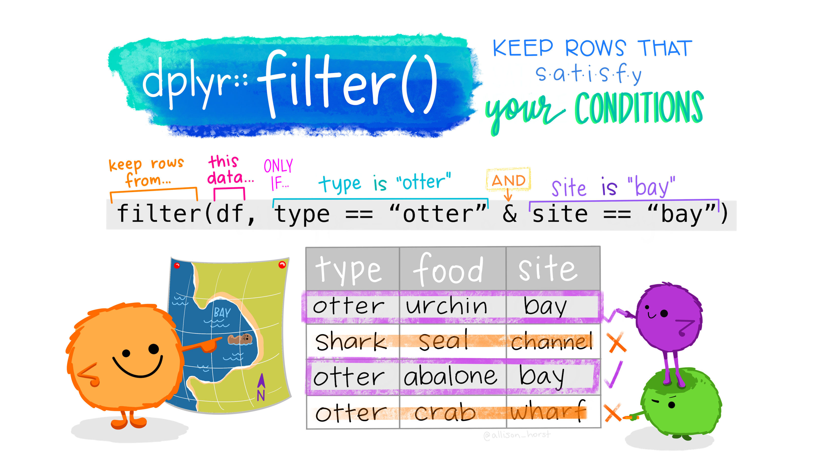
If we want to see the countries that also have an area that is less than the size of Ohio (116,098 km^2), we can also add that to our filter statement using the & operator.

factbook_2015 |> 
  filter(population_total > 11760000 & surface_area_sq_km < 116098)
# A tibble: 4 × 53
  country_name country_code population_total population_growth_annual_percent
  <chr>        <chr>                   <dbl>                            <dbl>
1 Guatemala    GTM                  15567419                            1.69 
2 Korea, Rep.  KOR                  51014947                            0.527
3 Netherlands  NLD                  16939923                            0.443
4 Sri Lanka    LKA                  21336697                            0.457
# ℹ 49 more variables: surface_area_sq_km <dbl>,
#   poverty_headcount_ratio_at_national_poverty_lines_percent_of_population <dbl>,
#   gni_atlas_method_current_us <dbl>,
#   gni_per_capita_atlas_method_current_us <dbl>,
#   gni_ppp_current_international <dbl>,
#   gni_per_capita_ppp_current_international <dbl>,
#   income_share_held_by_lowest_20_percent <dbl>, …

There are four countries that have more people than Ohio in a space that is less than Ohio.

2.1 Practice

How many countries have negative annual population growth? This variable is called population_growth_annual_percent.

Need a hint?

Try to filter for population_growth_annual_percent < 0.

Click for the solution
factbook_2015 |> 
  filter(population_growth_annual_percent < 0)
# A tibble: 34 × 53
   country_name           country_code population_total population_growth_annu…¹
   <chr>                  <chr>                   <dbl>                    <dbl>
 1 Albania                ALB                   2880703                   -0.291
 2 American Samoa         ASM                     51368                   -1.64 
 3 Armenia                ARM                   2878595                   -0.393
 4 Bosnia and Herzegovina BIH                   3524324                   -1.32 
 5 Bulgaria               BGR                   7177991                   -0.638
 6 Croatia                HRV                   4203604                   -0.824
 7 Greece                 GRC                  10820883                   -0.659
 8 Greenland              GRL                     56114                   -0.322
 9 Hungary                HUN                   9843028                   -0.238
10 Isle of Man            IMN                     83593                   -0.362
# ℹ 24 more rows
# ℹ abbreviated name: ¹​population_growth_annual_percent
# ℹ 49 more variables: surface_area_sq_km <dbl>,
#   poverty_headcount_ratio_at_national_poverty_lines_percent_of_population <dbl>,
#   gni_atlas_method_current_us <dbl>,
#   gni_per_capita_atlas_method_current_us <dbl>,
#   gni_ppp_current_international <dbl>, …

There are 34 countries that have a negative annual growth rate in 2015.

3 Choose columns with select()

Often you will want to pick only certain columns in your dataframe, and you can do this with the function select(). You can pick columns generally by:

  • their names
  • their position
  • characteristics of that column

If we want to know how the arguments to select() work, we can access the documentation material about the function.

?select()

Let’s first select columns by their names. Let’s pick just the country_name, population_total, and surface_area_sq_km.

factbook_2015 |> 
  select(country_name, population_total, surface_area_sq_km)
# A tibble: 217 × 3
   country_name        population_total surface_area_sq_km
   <chr>                          <dbl>              <dbl>
 1 Afghanistan                 33753499             652860
 2 Albania                      2880703              28750
 3 Algeria                     39543154            2381741
 4 American Samoa                 51368                200
 5 Andorra                        71746                470
 6 Angola                      28127721            1246700
 7 Antigua and Barbuda            89941                440
 8 Argentina                   43131966            2780400
 9 Armenia                      2878595              29740
10 Aruba                         104257                180
# ℹ 207 more rows

Those columns are also the 1st, 3rd, and 5th columns in our data frame, do we can select them by their indices, or by their location.

factbook_2015 |> 
  select(1, 3, 5)
# A tibble: 217 × 3
   country_name        population_total surface_area_sq_km
   <chr>                          <dbl>              <dbl>
 1 Afghanistan                 33753499             652860
 2 Albania                      2880703              28750
 3 Algeria                     39543154            2381741
 4 American Samoa                 51368                200
 5 Andorra                        71746                470
 6 Angola                      28127721            1246700
 7 Antigua and Barbuda            89941                440
 8 Argentina                   43131966            2780400
 9 Armenia                      2878595              29740
10 Aruba                         104257                180
# ℹ 207 more rows

In general I would recommend against this because its really hard to remember which column indices are which variables today, nevermind returning back to old code 1 year from now.

We can also select columns that are consecutive, using the : operator. Below I’m selecting the columns country_name through population_growth_annual_percent.

factbook_2015 |> 
  select(country_name:population_growth_annual_percent)
# A tibble: 217 × 4
   country_name        country_code population_total population_growth_annual_…¹
   <chr>               <chr>                   <dbl>                       <dbl>
 1 Afghanistan         AFG                  33753499                       3.12 
 2 Albania             ALB                   2880703                      -0.291
 3 Algeria             DZA                  39543154                       2.00 
 4 American Samoa      ASM                     51368                      -1.64 
 5 Andorra             AND                     71746                       0.174
 6 Angola              AGO                  28127721                       3.62 
 7 Antigua and Barbuda ATG                     89941                       0.787
 8 Argentina           ARG                  43131966                       1.08 
 9 Armenia             ARM                   2878595                      -0.393
10 Aruba               ABW                    104257                       0.638
# ℹ 207 more rows
# ℹ abbreviated name: ¹​population_growth_annual_percent

We can remove columns using the ! operator:

factbook_2015 |> 
  select(!country_code)
# A tibble: 217 × 52
   country_name       population_total population_growth_an…¹ surface_area_sq_km
   <chr>                         <dbl>                  <dbl>              <dbl>
 1 Afghanistan                33753499                  3.12              652860
 2 Albania                     2880703                 -0.291              28750
 3 Algeria                    39543154                  2.00             2381741
 4 American Samoa                51368                 -1.64                 200
 5 Andorra                       71746                  0.174                470
 6 Angola                     28127721                  3.62             1246700
 7 Antigua and Barbu…            89941                  0.787                440
 8 Argentina                  43131966                  1.08             2780400
 9 Armenia                     2878595                 -0.393              29740
10 Aruba                        104257                  0.638                180
# ℹ 207 more rows
# ℹ abbreviated name: ¹​population_growth_annual_percent
# ℹ 48 more variables:
#   poverty_headcount_ratio_at_national_poverty_lines_percent_of_population <dbl>,
#   gni_atlas_method_current_us <dbl>,
#   gni_per_capita_atlas_method_current_us <dbl>,
#   gni_ppp_current_international <dbl>, …

We can also select data based on its characteristics. We can select using selection helpers like:

For example, we might want each column that has anything to do with gross domestic product, or gdp. We can select all of the columns which contain the string “gdp” in their name. I’m also going to add country_name so we know what we’re working with.

factbook_2015 |> 
  select(country_name, contains("gdp"))
# A tibble: 217 × 15
   country_name     water_productivity_t…¹ gdp_current_us gdp_growth_annual_pe…²
   <chr>                             <dbl>          <dbl>                  <dbl>
 1 Afghanistan                       0.943    19134221645                  1.45 
 2 Albania                          12.4      11386853113                  2.22 
 3 Algeria                          20.9     187494000000                  3.2  
 4 American Samoa                   NA          673000000                  3.15 
 5 Andorra                          NA         2789881259                  1.43 
 6 Angola                          128.       90496420507                  0.944
 7 Antigua and Bar…                327.        1437755556                  1.45 
 8 Argentina                        15.8     594749000000                  2.73 
 9 Armenia                           3.23     10553337518                  3.20 
10 Aruba                            NA         2962907263                 -0.624
# ℹ 207 more rows
# ℹ abbreviated names:
#   ¹​water_productivity_total_constant_2015_us_gdp_per_cubic_meter_of_total_freshwater_withdrawal,
#   ²​gdp_growth_annual_percent
# ℹ 11 more variables: inflation_gdp_deflator_annual_percent <dbl>,
#   agriculture_forestry_and_fishing_value_added_percent_of_gdp <dbl>,
#   industry_including_construction_value_added_percent_of_gdp <dbl>, …

We can also select all column that meet a certain predicate. For example, we can pick all of the column that are of the type character.

factbook_2015 |> 
  select(where(is.character))
# A tibble: 217 × 2
   country_name        country_code
   <chr>               <chr>       
 1 Afghanistan         AFG         
 2 Albania             ALB         
 3 Algeria             DZA         
 4 American Samoa      ASM         
 5 Andorra             AND         
 6 Angola              AGO         
 7 Antigua and Barbuda ATG         
 8 Argentina           ARG         
 9 Armenia             ARM         
10 Aruba               ABW         
# ℹ 207 more rows

We can also combine selections using the & (and), | (or), and ! (not) operators. For example, if I want the columns about GNI but only the international ones I can:

factbook_2015 |> 
  select(starts_with("gni") & ends_with("international"))
# A tibble: 217 × 2
   gni_ppp_current_international gni_per_capita_ppp_current_international
                           <dbl>                                    <dbl>
 1                   77739869000                                     2300
 2                   33981401261                                    11800
 3                  541234000000                                    13690
 4                            NA                                       NA
 5                            NA                                       NA
 6                  190283000000                                     6760
 7                    1766297473                                    19640
 8                  848960000000                                    19680
 9                   30505448341                                    10600
10                    3718236361                                    35660
# ℹ 207 more rows

We can also use select() to order our columns, as the order we select them in dictates the order they will exist in our dataframe.

3.1 Practice

Come up with 3 different ways to select the columns about children, and make sure you also include a country column so you know what you’re looking at.

Need a hint?

Here are the columns that I’m considering to be about children:

[1] “country_name”
[17] “mortality_rate_under_5_per_1_000_live_births”
[18] “prevalence_of_underweight_weight_for_age_percent_of_children_under_5”
[19] “immunization_measles_percent_of_children_ages_12_23_months”
[20] “primary_completion_rate_total_percent_of_relevant_age_group”
[21] “school_enrollment_secondary_percent_gross”
[22] “school_enrollment_primary_and_secondary_gross_gender_parity_index_gpi”

Click for the solution

By name and for columns in a row, using the :.

factbook_2015 |> 
  select(country_name, 
         mortality_rate_under_5_per_1_000_live_births:
         school_enrollment_primary_and_secondary_gross_gender_parity_index_gpi)
# A tibble: 217 × 7
   country_name        mortality_rate_under_5_per_1_000…¹ prevalence_of_underw…²
   <chr>                                            <dbl>                  <dbl>
 1 Afghanistan                                       72.7                     NA
 2 Albania                                            9.6                     NA
 3 Algeria                                           25.3                     NA
 4 American Samoa                                    NA                       NA
 5 Andorra                                            3.6                     NA
 6 Angola                                            87.9                     19
 7 Antigua and Barbuda                               10.9                     NA
 8 Argentina                                         11.8                     NA
 9 Armenia                                           14.5                     NA
10 Aruba                                             NA                       NA
# ℹ 207 more rows
# ℹ abbreviated names: ¹​mortality_rate_under_5_per_1_000_live_births,
#   ²​prevalence_of_underweight_weight_for_age_percent_of_children_under_5
# ℹ 4 more variables:
#   immunization_measles_percent_of_children_ages_12_23_months <dbl>,
#   primary_completion_rate_total_percent_of_relevant_age_group <dbl>,
#   school_enrollment_secondary_percent_gross <dbl>, …

By index:

factbook_2015 |> 
  select(1, 17:22) 
# A tibble: 217 × 7
   country_name        mortality_rate_under_5_per_1_000…¹ prevalence_of_underw…²
   <chr>                                            <dbl>                  <dbl>
 1 Afghanistan                                       72.7                     NA
 2 Albania                                            9.6                     NA
 3 Algeria                                           25.3                     NA
 4 American Samoa                                    NA                       NA
 5 Andorra                                            3.6                     NA
 6 Angola                                            87.9                     19
 7 Antigua and Barbuda                               10.9                     NA
 8 Argentina                                         11.8                     NA
 9 Armenia                                           14.5                     NA
10 Aruba                                             NA                       NA
# ℹ 207 more rows
# ℹ abbreviated names: ¹​mortality_rate_under_5_per_1_000_live_births,
#   ²​prevalence_of_underweight_weight_for_age_percent_of_children_under_5
# ℹ 4 more variables:
#   immunization_measles_percent_of_children_ages_12_23_months <dbl>,
#   primary_completion_rate_total_percent_of_relevant_age_group <dbl>,
#   school_enrollment_secondary_percent_gross <dbl>, …

By name characteristics:

factbook_2015 |> 
  select(country_name, contains("under_5"), contains("children"),
         contains("primary"), contains("school"))
# A tibble: 217 × 7
   country_name        mortality_rate_under_5_per_1_000…¹ prevalence_of_underw…²
   <chr>                                            <dbl>                  <dbl>
 1 Afghanistan                                       72.7                     NA
 2 Albania                                            9.6                     NA
 3 Algeria                                           25.3                     NA
 4 American Samoa                                    NA                       NA
 5 Andorra                                            3.6                     NA
 6 Angola                                            87.9                     19
 7 Antigua and Barbuda                               10.9                     NA
 8 Argentina                                         11.8                     NA
 9 Armenia                                           14.5                     NA
10 Aruba                                             NA                       NA
# ℹ 207 more rows
# ℹ abbreviated names: ¹​mortality_rate_under_5_per_1_000_live_births,
#   ²​prevalence_of_underweight_weight_for_age_percent_of_children_under_5
# ℹ 4 more variables:
#   immunization_measles_percent_of_children_ages_12_23_months <dbl>,
#   primary_completion_rate_total_percent_of_relevant_age_group <dbl>,
#   school_enrollment_primary_and_secondary_gross_gender_parity_index_gpi <dbl>, …

These are just some ways!

4 Sorting data with arrange()

A nice helper function for looking at your data is arrange() which sorts your data.

We can sort our data based on how much forest (forest_area_sq_km) each country has.

factbook_2015 |> 
  arrange(forest_area_sq_km)
# A tibble: 217 × 53
   country_name             country_code population_total population_growth_an…¹
   <chr>                    <chr>                   <dbl>                  <dbl>
 1 Gibraltar                GIB                     32520                  0.209
 2 Monaco                   MCO                     36760                  1.78 
 3 Nauru                    NRU                     11185                  2.21 
 4 Qatar                    QAT                   2414573                  8.65 
 5 Curacao                  CUW                    157980                  1.32 
 6 Faroe Islands            FRO                     48816                  0.722
 7 Greenland                GRL                     56114                 -0.322
 8 Malta                    MLT                    445053                  2.39 
 9 Sint Maarten (Dutch par… SXM                     38825                  2.98 
10 Aruba                    ABW                    104257                  0.638
# ℹ 207 more rows
# ℹ abbreviated name: ¹​population_growth_annual_percent
# ℹ 49 more variables: surface_area_sq_km <dbl>,
#   poverty_headcount_ratio_at_national_poverty_lines_percent_of_population <dbl>,
#   gni_atlas_method_current_us <dbl>,
#   gni_per_capita_atlas_method_current_us <dbl>,
#   gni_ppp_current_international <dbl>, …

By default, arrange() sorts small to big, if we want to go from big to small we can set arrange(desc()) to sort by descending.

factbook_2015 |> 
  arrange(desc(forest_area_sq_km))
# A tibble: 217 × 53
   country_name       country_code population_total population_growth_annual_p…¹
   <chr>              <chr>                   <dbl>                        <dbl>
 1 Russian Federation RUS                 144640716                        0.279
 2 Brazil             BRA                 205188205                        0.846
 3 Canada             CAN                  35704498                        0.760
 4 United States      USA                 320738994                        0.736
 5 China              CHN                1379860000                        0.581
 6 Australia          AUS                  23815995                        1.44 
 7 Congo, Dem. Rep.   COD                  78656904                        3.39 
 8 Indonesia          IDN                 259091970                        1.11 
 9 Peru               PER                  30711863                        1.17 
10 India              IND                1322866505                        1.19 
# ℹ 207 more rows
# ℹ abbreviated name: ¹​population_growth_annual_percent
# ℹ 49 more variables: surface_area_sq_km <dbl>,
#   poverty_headcount_ratio_at_national_poverty_lines_percent_of_population <dbl>,
#   gni_atlas_method_current_us <dbl>,
#   gni_per_capita_atlas_method_current_us <dbl>,
#   gni_ppp_current_international <dbl>, …

It’s not too surprising that the biggest countries in forest-feasible lattitudes have the most forest.

We can also add select() into our pipe, so that we don’t have to scroll so far to see what the actual amount of forest is.

factbook_2015 |> 
  select(country_name, surface_area_sq_km, forest_area_sq_km) |> 
  arrange(desc(forest_area_sq_km))
# A tibble: 217 × 3
   country_name       surface_area_sq_km forest_area_sq_km
   <chr>                           <dbl>             <dbl>
 1 Russian Federation           17098250          8149305.
 2 Brazil                        8515770          5038848 
 3 Canada                        9879750          3471157.
 4 United States                 9831510          3100950 
 5 China                         9562911          2102942.
 6 Australia                     7741220          1330945 
 7 Congo, Dem. Rep.              2344860          1316621.
 8 Indonesia                     1913580           950279 
 9 Peru                          1285220           731945.
10 India                         3287260           708280 
# ℹ 207 more rows

Wow almost 50% of Russia is forested.

4.1 Practice

Which countries have the lowest cell phone subscriptions? mobile_cellular_subscriptions_per_100_people

Need a hint?

You can use the function arrange() to sort your columns. The default arranging is from low to high, so if you want to go from high to low, you can set arrange(desc()).

Click for the solution
factbook_2015 |> 
  select(country_name, mobile_cellular_subscriptions_per_100_people) |> 
  arrange(mobile_cellular_subscriptions_per_100_people)
# A tibble: 217 × 2
   country_name              mobile_cellular_subscriptions_per_100_people
   <chr>                                                            <dbl>
 1 Korea, Dem. People's Rep.                                         12.8
 2 Eritrea                                                           14.2
 3 Micronesia, Fed. Sts.                                             20.6
 4 Central African Republic                                          25.8
 5 South Sudan                                                       25.9
 6 Cuba                                                              29.4
 7 Djibouti                                                          31.2
 8 Marshall Islands                                                  31.4
 9 Kiribati                                                          35.1
10 Chad                                                              38.7
# ℹ 207 more rows
Back to top