Reproducibility recommendations: Code styling

Recommendations on code styling to improve the reproducibility of your research

reproducibility

Author

Horacio Lopez-Nicora

Published

October 6, 2025

1 Introduction

Good coding style is like correct punctuation: you can manage without it, butitsuremakesthingseasiertoread. [R for Data Science (2e)]

Welcome to this Code Club OSU session on Code Styling in R. Whether you’re just starting out with R or looking to improve the readability and consistency of your code, this session is designed to give you practical, beginner-friendly guidance on writing clean and professional R code. Code styling is more than just aesthetics, it’s about making your code easier to understand, debug, and share with others. In collaborative environments like research labs, classrooms, or open-source projects, consistent style helps everyone stay on the same page.

Today, we’ll explore key principles from the tidyverse style guide and the R for Data Science workflow/style chapter, and apply them using real datasets like palmerpenguins.

By the end of this session, you’ll be able to recognize good style, apply it to your own code, and understand why it matters. Let’s dive in!

Before we start, let’s quickly build on what we covered last session about organizing our code. Now, go ahead and load the tidyverse and janitor packages. If you haven’t installed them yet, install them first.

Code

# LOAD PACKAGES

# install.packages("janitor")
library(janitor) # To fix column names with clean_names() (version 2.2.1)

#install.packages("janitor")
library(tidyverse) # Data summarizing, plotting, and writing (version 2.0.0)

2 Why Code Style Matters

When writing code, especially in a collaborative or academic setting, style is not just a matter of personal preference, it’s a matter of clarity and professionalism.

Well-styled code is easier to read, debug, and maintain. It helps others understand your logic without needing extensive explanations. Inconsistent or messy code can slow down projects, introduce errors, and make collaboration frustrating. By following a consistent style guide, like the tidyverse style guide, you ensure that your code communicates clearly and efficiently. Today, we’ll learn how to make our R code clean, readable, and consistent; skills that will serve you well in research, coursework, and data science projects.

3 Naming Conventions: Human-Readable & Machine-Readable

One of the first steps toward clean code is choosing good names for your variables and functions. In R, we recommend using snake_case—lowercase letters with underscores separating words. For example, penguin_summary is much clearer than something like df1 or temp.

Good names describe what the object contains or does, making your code self-documenting. Avoid abbreviations unless they’re widely understood, and don’t be afraid to use longer names if they improve clarity. Think of naming as labeling your thoughts, make it easy for someone else (or future you) to understand what each part of your code is doing.

# Messy Example
df1 <- penguins
temp <- group_by(df1, species)
result <- summarise(temp, mean(body_mass, na.rm = TRUE))

# Styled Example
penguin_summary <- penguins |> 
  group_by(species) |> 
  summarise(avg_mass = mean(body_mass, na.rm = TRUE))

# Style notes:
# - Use descriptive names: 'penguin_summary' instead of 'df1' or 'temp'
# - Use snake_case consistently
# - Avoid vague or temporary names

Good names serve two audiences:

Humans: other programmers (or your future self) need to understand what the code does quickly.
Machines: R and other tools need names that are valid, unambiguous, and free of spaces or special characters.

3.1 Human-Readable

Names should clearly describe the content or purpose of the object.
Avoid abbreviations that aren’t widely understood.

# We immediately know what it represents:
avg_flipper_length <- mean(penguins$flipper_len, na.rm = TRUE)

# Avoid vague or cryptic names:
x <- mean(penguins$flipper_len)

3.2 Machine-Readable

Avoid spaces, special characters, or punctuation in names.
Column names imported from CSVs are often not machine-friendly:

#"Flipper Length (mm)" → contains spaces and parentheses 

# Use snake_case and letters/numbers/underscores only:
flipper_length_mm

3.3 Balancing Both

Aspect	Recommendation
Human readability	Use descriptive, clear names, readable words, meaningful abbreviations
Machine readability	Use snake_case, no spaces/special characters, consistent casing
Example	`avg_bill_length` ✅ vs `Avg.Bill.Length` ❌

Tools like janitor::clean_names() make column names both human- and machine-readable:

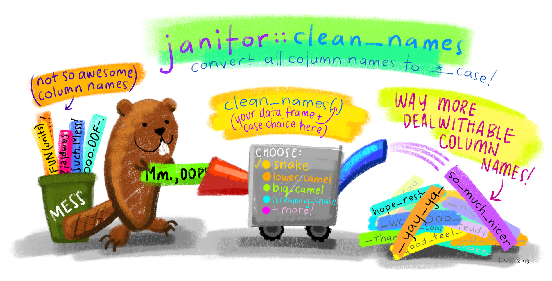
Using janitor::clean_names() at the start of a data analysis project is a simple step that prevents a lot of frustration later. Real-world datasets often come with inconsistent, messy column names—things like spaces, capital letters, punctuation, or mixed naming styles. These names can slow you down when writing code, force you to use backticks, and break the flow of tidyverse functions.

By cleaning names immediately, you convert everything to consistent, machine-friendly, snake_case column names that are easy to type, reference, and style. It also supports cleaner pipelines, improves readability, and aligns with best practices for reproducible and collaborative code.

Code

# MESSY Code

# Examine dataset
penguins_raw |> glimpse()

# Select variables of interes
penguins_raw |> select(`Body Mass (g)`, Sex, `Date Egg`)

# STYLED Code

# Use janitor::clean_names and select same variables
penguins_raw |> clean_names() |> glimpse()
penguins_raw |> clean_names() |> select(body_mass_g, sex, date_egg)

4 Pipes and Indentation

The pipe operator (|>) is one of the most powerful tools in the tidyverse. It allows you to write code that reads like a sequence of actions: take this data, do this, then do that. Each step in a pipeline should be indented on a new line, making the flow of logic easy to follow. For example, when summarizing data, you might start with penguins |>, then indent group_by(species), and follow with summarise(...). This structure helps you and others quickly scan and understand the transformation. Indentation is not just about aesthetics—it’s about making your code readable and maintainable.

Lets’ look at some examples:

Example 1: Filtering and Summarizing

Code

# ❌ BAD STYLE: Cramped, no indentation, unclear naming
x <- penguins |> filter(species=="Adelie") |> group_by(island) |> summarise(avg=mean(body_mass,na.rm=TRUE))

# ✅ GOOD STYLE: Clear naming, spacing, indentation, and comments
adelie_summary <- penguins |> 
  filter(species == "Adelie") |> # Filter to Adelie penguins
  group_by(island) |>            # Group by island
  summarise(avg_mass = mean(body_mass, na.rm = TRUE))  # Calculate average body mass

Example 2: Mutate and Arrange

Code

# ❌ BAD STYLE: Semicolon chaining, inconsistent naming
penguins2<-mutate(penguins,bmi=body_mass/bill_len);arrange(penguins2,bmi)

# ✅ GOOD STYLE: Pipe used throughout, clear naming, spacing, and indentation
penguins_bmi <- penguins |> 
  mutate(bmi = body_mass / bill_len) |> # Create BMI variable
  arrange(bmi)                                  # Sort by BMI

Example 3: Summarise Misalignment

Code

# ❌ BAD STYLE: Misaligned summarise arguments
penguins |> 
  group_by(species) |> 
  summarise(avg_mass = mean(body_mass, na.rm = TRUE), 
  count = n())

# ✅ GOOD STYLE: Each summary on its own line, aligned
penguins |> 
  group_by(species) |> 
  summarise(
    avg_mass = mean(body_mass, na.rm = TRUE),
    count = n()
  )

Example 4: Broken Pipe Chain

Code

# ❌ BAD STYLE: Pipe chain is broken
penguins |> 
  group_by(species)
summarise(avg_mass = mean(body_mass, na.rm = TRUE))

# ✅ GOOD STYLE: Pipe chain is continuous
penguins |> 
  group_by(species) |> 
  summarise(avg_mass = mean(body_mass, na.rm = TRUE))

5 Spacing and Alignment

Consistent spacing around operators and arguments improves readability. For example, write x = 5 instead of x=5, and align similar lines when possible. This makes patterns in your code easier to spot and reduces cognitive load. When writing multiple lines of similar code, aligning them vertically can help highlight differences and similarities. Think of spacing as visual punctuation, it guides the reader’s eye and helps them parse your code more easily. Avoid cramming everything into one line; give your code room to breathe.

Example 1: Assignment and Function Calls

Code

# ❌ BAD STYLE: No spacing, cramped code
penguins_summary<-penguins|>group_by(species)|>summarise(avg=mean(body_mass,na.rm=TRUE))

# ✅ GOOD STYLE: Proper spacing and alignment
penguins_summary <- penguins |> 
  group_by(species) |> 
  summarise(avg_mass = mean(body_mass, na.rm = TRUE))

# Style notes:
# - Use spaces around assignment (<-), pipes (|>), and function arguments (=)
# - Align each step of the pipeline on a new line
# - Use descriptive variable and column names

Example 2: Multiple Arguments in `summarise()`

Code

# ❌ BAD STYLE: Arguments crammed together
penguins |> group_by(species) |> summarise(avg=mean(body_mass,na.rm=TRUE),count=n())

# ✅ GOOD STYLE: Each argument on its own line, aligned
penguins |> 
  group_by(species) |> 
  summarise(
    avg_mass = mean(body_mass, na.rm = TRUE),
    count = n()
  )

# Style notes:
# - Each summary metric is on its own line
# - Arguments are aligned for readability

6 Inline Comments

Comments are your opportunity to explain why your code does what it does. While code should be self-explanatory through good naming and structure, comments provide context that might not be obvious. For example, # remove NA values tells the reader why na.rm = TRUE is used. Avoid redundant comments like # load data when the code already says library(palmerpenguins). Instead, focus on explaining decisions, assumptions, or non-obvious steps. Comments should be brief, relevant, and placed directly above or beside the code they refer to.

Example 1: No Comments or Unhelpful Comments

Code

# ❌ BAD STYLE: No explanation or vague comment
penguins |> 
  filter(species == "Chinstrap") |> 
  summarise(mean(flipper_len, na.rm = TRUE))  # summary

# ✅ GOOD STYLE: Clear, helpful inline comments
penguins |> 
  filter(species == "Chinstrap") |>                 # Focus on Chinstrap penguins
  summarise(avg_flipper = mean(flipper_len, na.rm = TRUE))  # Calculate average flipper length

# Style notes:
# - Comments explain *why* or *what* is being done
# - Avoid stating the obvious or repeating the code

Example 2: Misplaced or Redundant Comments

Code

# ❌ BAD STYLE: Redundant and misplaced comments
# This is a filter
penguins |> 
  filter(species == "Gentoo") |> 
  # This is a summarise
  summarise(mean(body_mass, na.rm = TRUE))

# ✅ GOOD STYLE: Concise and well-placed comments
penguins |> 
  filter(species == "Gentoo") |>                    # Filter for Gentoo penguins
  summarise(avg_mass = mean(body_mass, na.rm = TRUE))  # Calculate average body mass

7 Plotting with Style

Visualizations are a key part of data analysis, and styling your plots is just as important as styling your code. Use clear labels for axes and titles, choose readable color schemes, and structure your ggplot code with indentation for each layer. For example, start with ggplot(...), then indent geom_boxplot(...), labs(...), and theme_minimal(). This makes it easy to see how the plot is constructed. Avoid cluttered plots, simplicity and clarity should guide your design choices. Well-styled plots communicate insights effectively and make your work look polished.

Example 1: Cramped and Unlabeled Plot

Code

# ❌ BAD STYLE: No labels, no spacing
ggplot(penguins, aes(species, body_mass)) + geom_boxplot()

# ✅ GOOD STYLE: Clear labels, spacing, and structure
ggplot(penguins, aes(x = species, y = body_mass)) +
  geom_boxplot(fill = "lightblue") +
  labs(
    title = "Body Mass by Species",
    x = "Species",
    y = "Body Mass (g)"
  ) +
  theme_minimal()

# Style notes:
# - Use `labs()` to label axes and title
# - Indent each layer of the plot
# - Use readable color names and themes

Example 2: Overly Complex One-Liner

Code

# ❌ BAD STYLE: Everything in one line, hard to read
ggplot(penguins,aes(x=species,y=flipper_len,fill=sex))+geom_violin()+theme_minimal()+labs(title="Flipper Length",x="Species",y="Length")

# ✅ GOOD STYLE: Structured and readable
ggplot(penguins, aes(x = species, y = flipper_len, fill = sex)) +
  geom_violin() +
  labs(
    title = "Flipper Length by Species and Sex",
    x = "Species",
    y = "Flipper Length (mm)",
    fill = "Sex"
  ) +
  theme_minimal()

# Style notes:
# - Each ggplot layer is on its own line
# - Labels are clear and informative
# - Code is easy to scan and modify

8 Interactive Code Styling with `lintr` and `styler`

As you begin writing more R code, it’s helpful to use tools that automatically check and improve your code style. Two popular packages for this are lintr and styler. These tools help you write cleaner code by identifying style violations (lintr) and automatically reformatting code (styler) to follow tidyverse conventions.

These tools are especially useful in teaching, collaborative projects, and when preparing code for publication or sharing. Let’s look at how each works with examples.

# INSTALL PACKAGES
install.packages("lintr")
install.packages("styler")

# LOAD PACKAGES
library(lintr)
library(styler)

8.1 Using `lintr` to Check Code Style

lintr is like a spell-checker for your code. It scans your scripts and flags issues such as inconsistent spacing, bad naming, or improper indentation.

Example 1: Lint a messy code snippet

Code

styler::style_text("x <- 1+1")

lint(text = "penguins |>filter(species=='Adelie')|>summarise(mean(body_mass,na.rm=TRUE))")

# Output (example):
# - Missing spaces around operators
# - Pipe not followed by a space

Example 2: Lint a messy code for data viz

Code

lint(text = "ggplot(penguins,aes(species,body_mass))+geom_boxplot()")

# Output (example):
# - Missing spaces around operators
# - Layers not followed by a space

8.2 Using `styler` to Check Code Style

styler is like an auto-correct tool, it reformats your code to match a consistent style guide, such as the tidyverse style.

Example 1: Style a messy pipe chain

Code

style_text("penguins |>filter(species=='Adelie')|>summarise(mean(body_mass,na.rm=TRUE))")

# Output:
# penguins |> 
#   filter(species == "Adelie") |>

Example 2: Style a cluttered ggplot call

Code

style_text("penguins|>ggplot(aes(species,body_mass))+geom_boxplot()")

# Output:
# penguins |> ggplot(aes(species, body_mass_g)) +
#   geom_boxplot()

1 Introduction

2 Why Code Style Matters

3 Naming Conventions: Human-Readable & Machine-Readable

3.1 Human-Readable

3.2 Machine-Readable

3.3 Balancing Both

4 Pipes and Indentation

Example 1: Filtering and Summarizing

Example 2: Mutate and Arrange

Example 3: Summarise Misalignment

Example 4: Broken Pipe Chain

5 Spacing and Alignment

Example 1: Assignment and Function Calls

Example 2: Multiple Arguments in summarise()

6 Inline Comments

Example 1: No Comments or Unhelpful Comments

Example 2: Misplaced or Redundant Comments

7 Plotting with Style

Example 1: Cramped and Unlabeled Plot

Example 2: Overly Complex One-Liner

8 Interactive Code Styling with lintr and styler

8.1 Using lintr to Check Code Style

Example 1: Lint a messy code snippet

Example 2: Lint a messy code for data viz

8.2 Using styler to Check Code Style

Example 1: Style a messy pipe chain

Example 2: Style a cluttered ggplot call

Example 2: Multiple Arguments in `summarise()`

8 Interactive Code Styling with `lintr` and `styler`

8.1 Using `lintr` to Check Code Style

8.2 Using `styler` to Check Code Style