# Remove 3 outliers that were identified by XYZ:
data_filt <- data |> filter(sample_id %in% outliers) Reproducibility recommendations: Code structure
Recommendations on code structure to improve the reproducibility of your research
reproducibility
1 Introduction
Have you struggled with R scripts whose size spins out of control, not being sure where items in your environment came from, or no longer being able to run the code in your script? Then, the recommendations that we’ll discuss in today’s Code Club session should come in handy.
We’ll cover a variety of best-practice techniques on how to structure your R scripts and Quarto (/ R Markdown) documents. In the text below, I will mostly refer to scripts, but these recommendations also apply to Quarto, sometimes in slightly modified form. The recommendations are:
- Use explanatory comments and divide your script into sections
- Write self-contained scripts
- Put the following at the top of your script:
- A comment describing the function of your script, and code to:
- Load packages
- Define input and output files
- Settings for your analysis
- Don’t let your scripts get too long
- Don’t repeat yourself – as in, don’t copy and paste blocks of code when you need to repeat an action
As we go through these recommendation, let’s have a scenario in mind where you are working on R code for your paper’s final figures.
2 Use comments and divide your script into sections
For future you and others who may read your code, make extensive use of comments to explain what your code does and why, e.g:
# Turn `strawberry_line` into a factor to ensure proper ordering in the plots:
data <- data |> mutate(strawberry_line = factor(strawberry_line, levels = line_order))
In RStudio, you can use a special kind of comment to divide your code into sections:
# A: SETUP ---------------------------------------------------------------------
# This section will load packages and define input and output files.
# Step 1: load packages
# ...R code...
# B: DATA WRANGLING ------------------------------------------------------------
# This section will wrangle the miserably formatted data into a shape
# that can be used for plotting.
# Step 1: XYZ
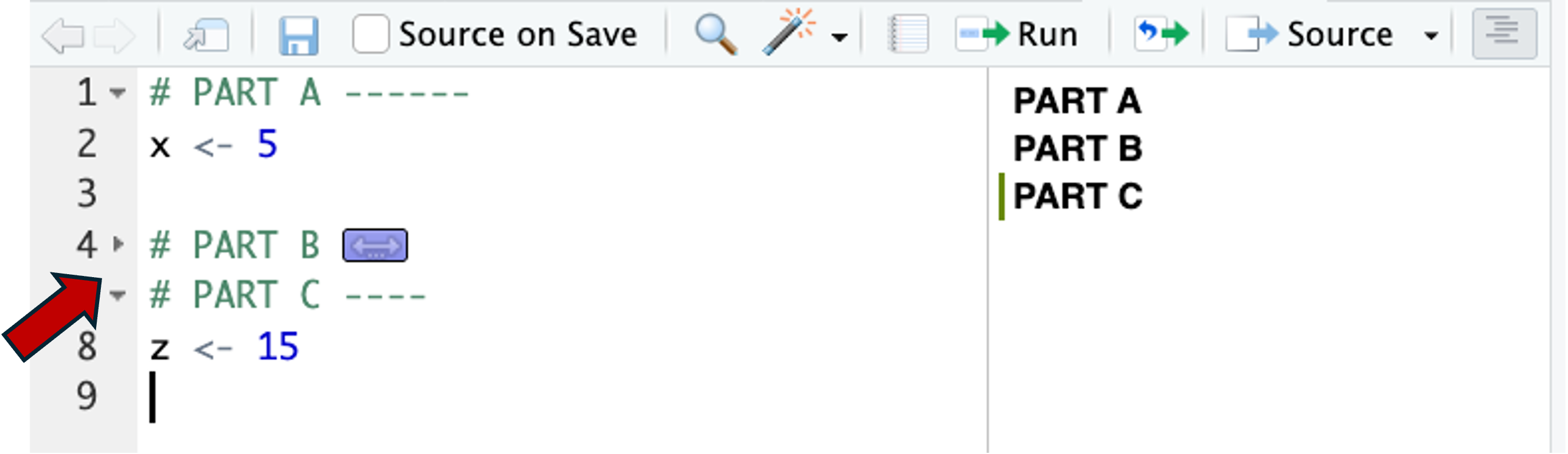
# ...R code...Adding 4 or more dashes (-) at the end of a comment line will make RStudio interpret it as a section header and:
- Show an outline of your document if you click on the icon highlighted with a red arrow in the screenshot below:
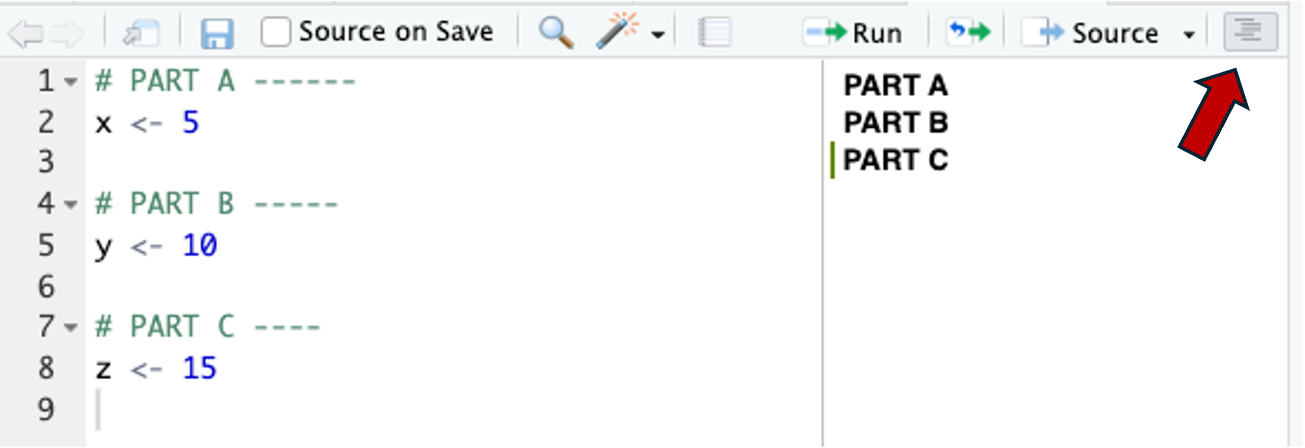
In the outline, allow you to click on the headers to navigate to that part of your script
Allow you to collapse sections by clicking on the little arrow icons in the margin:
3 Write self-contained scripts
3.1 You should be able to run your script in a fresh R environment
You should always be able to run the code in your script from start to finish, starting from a completely fresh (empty) R environment. This means that your script should never use, for example:
- R objects that were not created by it
- Packages that were not loaded by it
- Custom functions that were not created or loaded by it
In other words, your script should never just “continue on” from another script, or assume that packages have been loaded beforehand/elsewhere, and so on.
3.2 Don’t include code you don’t actually want to run
This also applies to code that had a purpose in earlier runs of the script, but does no longer. For example, installing packages is a one-time setup step that you won’t want to rerun every time you work on your script. The R functions that do this should therefore not be included in the script.
# If you include install.packages() in your script, running the script
# from start to finish means re-installing the package every time
install.packages(tidyverse)
library(tidyverse)
Instead, you ideally use a separate “install” script or document with installation and perhaps other one-time setup steps. Alternatively, you may add comments in your script with such information:
# Installed with install.packages("tidyverse") on 2025-09-29 (v 2.0.0)
library(tidyverse)
3.3 Avoid/minimize commented-out code
In general, though, avoid or at least minimize having code that is “commented out”. While commenting out code can be very useful when you’re experimenting, don’t keep it in your script any longer than necessary. An example of commented-out code:
# Only keep ripe strawberries
data <- data |> filter(strawberry_color != "green")
# data <- data |> select(!some_column)

# Create Fig. 1
ggplot(data, ...)
The above code should run without error whether you include or exclude the commented-out line. Without an explanation, this may therefore be confusing to future you, your collaborators, etc.
Any commented-out code that you are keeping around for longer should be clearly annotated – explain why it is commented out and why are you keeping it around:
# Only keep ripe strawberries
data <- data |> filter(strawberry_color != "green")

# 'some_column' column may need to be removed for final outputs,
# but I got a warning I didn't understand when removing it - keeping this for now
# data <- data |> select(!some_column)

# Create Fig. 1
ggplot(data, ...)
3.4 Running your script from start to finish should produce all needed outputs
You may have a scenario where you need to run a large chunk of code, or perhaps the entire script, multiple times. For example, once for each of several input files or each of several different parameter thresholds. You may be inclined to include this as a “setting” of the top of the script, commenting out the other possibilities.
# I ran the code below for both of these experiments:
input_file <- "data/experiment01.tsv"
output_plot <- "results/exp01_plot.png"
#input_file <- "data/experiment02.tsv"
#output_plot <- "results/exp02_plot.png"
Or to just include a comment like this:
p_value <- 0.05 # Ran analysis below also with p of 0.01 and 0.10Avoid these kind of constructs as well, because simply running your script in its entirety should produce all the outputs that are needed. Also see the “Don’t repeat yourself” recommendation further down.
3.5 Restart R regularly
If at all possible, try to restart R regularly and start over by running your code from the beginning of the script in a fresh environment. This ensures that your script is indeed self-contained.
Restarting R will also alert you to the all-too-common situation of:
- Having code in your script that no longer works because of changes you made, but
- You fail to notice this because your R environment still reflects the old code.
One typical cause of this situation is when you rename an object. The more regularly you restart, the less risk you run of getting into this situation and then having a really hard time figuring out what changed.
Tip
If it seems prohibitive to restart R regularly because there is so much code to rerun, and/or that code takes a long time to run, you should consider splitting your script into different parts. See the section “Don’t let your scripts get too long” below.
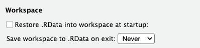
To make sure that R starts in a fresh environment upon restarting, use the following settings in RStudio (Tools > Global Options) – uncheck the the “Restore …” box and set the other option to “Never”:
To actually restart R, click Session > Restart R:
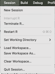
Pay attention to the keyboard shortcut that is shown there, and try to get used to using that!
Exercise: Restart R
Make sure you have a couple of things in your R environment.
Restart R – test the keyboard shortcut.
Check that your R environment is now empty.
4 Put these things at the top of your script
4.1 A comment describing the function of your script
For example:
# Author: Jane Doe
# Date: 2025-09-29, with edits on 2025-10-05
# Project: ~/Documents/thesis/strawberry-experiment
# Purpose: Create a figure to ...
If you’re using a Quarto document instead, most of this kind of information will likely go into the YAML header.
4.2 Loading packages
Don’t load packages throughout your script, and certainly don’t omit the code to load packages as explained above. Instead, load all packages at the top of the script – for example:
# Load packages
library(tidyverse)   # Data wrangling and plotting (v 2.0.0)
library(patchwork)   # Creating multi-panel figures (v 1.3.2)
library(ggforce)     # For the facet_zoom() function (v 0.5.0)
library(janitor)     # Variable name cleaning (v 2.2.1)
library(here)        # Creating file paths (v 1.0.1)
The above example also includes a brief explanation of what each package is used for, and which version is (or should be / was) loaded.
TipMore about recording R package versions (Click to expand)
To report package versions, you can also run the sessionInfo() function:
sessionInfo()R version 4.5.1 (2025-06-13)
Platform: aarch64-apple-darwin20
Running under: macOS Sequoia 15.7
Matrix products: default
BLAS: /Library/Frameworks/R.framework/Versions/4.5-arm64/Resources/lib/libRblas.0.dylib
LAPACK: /Library/Frameworks/R.framework/Versions/4.5-arm64/Resources/lib/libRlapack.dylib; LAPACK version 3.12.1
locale:
[1] en_US.UTF-8/en_US.UTF-8/en_US.UTF-8/C/en_US.UTF-8/en_US.UTF-8
time zone: America/New_York
tzcode source: internal
attached base packages:
[1] stats graphics grDevices utils datasets methods base
loaded via a namespace (and not attached):
[1] htmlwidgets_1.6.4 compiler_4.5.1 fastmap_1.2.0 cli_3.6.5
[5] tools_4.5.1 htmltools_0.5.8.1 rstudioapi_0.17.1 yaml_2.3.10
[9] rmarkdown_2.29 knitr_1.50 jsonlite_2.0.0 xfun_0.53
[13] digest_0.6.37 rlang_1.1.6 evaluate_1.0.4 It is particularly convenient to include that code in a Quarto document – there, you can put this function all the way at the end, so its output will be included in the rendered document. In an R script, you could include the following to save the info to file:
writeLines(capture.output(sessionInfo()), "sessionInfo.txt")4.3 Settings
If your script has any key settings for your analysis, especially ones you may want to change later on, you should also include these at the top of your script. For example:
# General settings
p_value <- 0.01
logfold_change <- 1
some_threshold <- 25
remove_outliers <- TRUE

# Plot settings
theme_set(theme_minimal(base_size = 13))
treatment_colors <- c(control = "gray50", mock = "gray20", inoculated = "blue")
This may also include miscellaneous things like setting the random seed, which makes functions with random sampling reproducible:
# Set the random seed for sampling with function rnorm()
set.seed(1)
4.4 Defining input and output files
It’s a good idea to define all of a script’s input and output files using variables at the top of the script – for example:
Input files:
# Define the input files
data_file <- "data/strawberries.tsv"
sampledata_file <- "data/meta/samples.tsv"
Output files:
# Define and create the output dir
outdir <- "results/plots"
dir.create(outdir, showWarnings = FALSE, recursive = TRUE)

# Define the output files
boxplot_file <- here(outdir, "boxplot.png")
scatterplot_file <- here(outdir, "scatterplot.png")
Then, you would use these variables when reading and writing later on:
data <- read_tsv(data_file)
ggsave(boxplot_file)
# Etc.
4.5 Putting it together
All in all, the top section of your script may look something like this:
# Author: Jane Doe
# Date: 2025-09-29, with edits on 2025-10-05
# Project: ~/Documents/thesis/strawberry-experiment
# Purpose: Create a figure to ...

# SETUP ------------------------------------------------------------------------
# Load packages
library(tidyverse)   # (v 2.0.0)
library(patchwork)   # Creating multi-panel figures (v 1.3.2)
library(ggforce)     # For the facet_zoom() function (v 0.5.0)
library(janitor)     # Variable name cleaning (v 2.2.1)
library(here)        # Creating file paths (v 1.0.1)

# General settings
p_value <- 0.01
logfold_change <- 1
some_threshold <- 25
remove_outliers <- TRUE

# Plot settings
theme_set(theme_minimal(base_size = 13))
treatment_colors <- c(control = "gray50", mock = "gray20", inoculated = "blue")

# Define the input files
data_file <- "data/strawberries.tsv"
sampledata_file <- "data/meta/samples.tsv"

# Define and create the output dir
outdir <- "results/plots"
dir.create(outdir, showWarnings = FALSE, recursive = TRUE)

# Define the output files
boxplot_file <- here(outdir, "boxplot.png")
scatterplot_file <- here(outdir, "scatterplot.png")
Exercise: Restructuring a script
Restructure this script according to the recommendations above:
library(janitor)
data <- iris |>
  clean_names()
head(data)

library(ggplot2)
data$sepal_length[1:10]
ggplot(data, aes(x = sepal_length, y = petal_length)) +
  geom_point() #+
  #geom_line()
ggsave("results/plots/plot.png")

library(dplyr)
data_summary <- data |>
  summarize(mean_sepal_length = mean(sepal_length), .by = species)
library(readr)
write_tsv(data_summary, here("results/data_summary.tsv"))
Click here for some pointers
- Note that there are currently no comments or sections in the script
- Do you think
head(data)and a simmilar line should be in your final script? - The code currently assumes that the dir
results/plotsexists. - Could you load ggplot2, dplyr, and readr, with a single
library()call?
Click here for a possible solution
Note that in the suggestion below, I removed the head(data) and data$sepal_length[1:10] lines. These are lines that aren’t really a problem to keep in, but unless they come with a clear directive, are a kind of clutter – you are better of just typing these kinds of things directly in the Console.
# SETUP ------------------------------------------------------------------------
# Load packages
library(janitor)    # To fix column names with clean_names() (version X)
library(tidyverse)  # Data summarizing, plotting, and writing (version X)

# Make sure the output dir(s) exist
outdir <- "results/plots"
dir.create(outdir, showWarnings = FALSE, recursive = TRUE)

# Define the output files
plotfile <- "results/plots/plot.png"
data_summary_file <- "results/data_summary.tsv"

# LOAD AND PREP THE DATA -------------------------------------------------------
data <- iris |>
  clean_names()

# VISUALIZE THE DATA -----------------------------------------------------------
ggplot(data, aes(x = sepal_length, y = petal_length)) +
  geom_point()
ggsave(plotfile)

# SUMMARIZE THE DATA -----------------------------------------------------------
data_summary <- data |>
  summarize(mean_sepal_length = mean(sepal_length), .by = species)
write_tsv(data_summary, data_summary_file))
5 Don’t let your scripts get too long
Your scripts should not become too long or they will become very hard to understand and to manage. And if you are working with Quarto instead, they will take a long time to render and are much more likely to fail while rendering. It is much better to have relatively short, modular scripts, each with a clear purpose.
It hopefully seems like common sense to start a new script when you switch to an unrelated analysis that uses different data, even if this is within the same project. But it is not always this easy.
5.1 Splitting “continuous” scripts
As an analysis expands and expands, it is often most convenient to just keep adding things to the same script. Such as when:
- All analyses work with the same data, and the script first does extensive data processing for all analyses; or
- Some or all analyses are not independent but more like a pipeline, where the outputs of step A are used in step B, the outputs of step B are used in step C, and so on.
However, also in such scenarios, it is a good idea to not let a single script get too long, and to start a new script sooner rather than later. To do this in practice, you will need to write intermediate outputs to file, and load them in your next script.
Consider an example where we do a whole bunch, perhaps hundreds of lines, of data prepping, and this data is then used by an big analysis and one or more plots. Whenever you work on on the plot, you find yourself rerunning the data prepping code, and skipping the analysis code. Perhaps this can be split into three scripts:
- Data prep
- Data analysis
- Data visualization
In practice, in much abbreviated form, this could look something like this:
# Shared data prep
data_prepped <- data |>
  filter(...) |>
  mutate(...) |>
  select(...)

# Analysis
lm(..., data_prepped)

# Plot
data_prepped |>
  ggplot(...)
Which can be split as follows:
Script 1 – Data prep:
data_prepped <- data |>
  filter(...) |>
  mutate(...) |>
  select(...)
write_tsv(data_prepped, "<data-prepped-file>")
Script 2 – Data analysis:
data_prepped <- read_tsv("<data-prepped-file>")

lm(..., data_prepped)
Script 3 – Data visualization:
data_prepped <- read_tsv("<data-prepped-file>")

data_prepped |>
  ggplot(...)
As you can see, this does mean you need more code in total. But in the long run, having smaller scripts is often worth it!
NoteHave more complicated objects?
If your intermediate output includes more complex R objects that are not easily saved to TSV/CSV and similar files, you can use a pair of functions to save and load R objects “as is”. For example:
Saving the object to file:
saveRDS(some_complicated_object, "object.RDS")Loading the object from file:
some_complicated_object <- readRDS("object.RDS")
6 Don’t repeat yourself (DRY)
If you find yourself…
- Copying and pasting large chunks of code only to make minor edits to the pasted code, or
- Using the abovementioned strategy where you run the code in your script multiple times after changing a setting or input file
…then you may want to learn about techniques that can help you avoid repeating yourself. One of the best ways of doing so is to write your own functions, and then iterate with “functional programming” functions (map(), apply-family, etc) or loops to elegantly run these functions multiple times.
How to do this in practice in beyond the scope of this session, but we do have a previous series of Code Club sessions about this.