Iterating part II: writing custom functions and `purrr:map()`

Instead of using loops, we can iterate with functions!

functions

functional programming

purrr

Author

Jessica Cooperstone

Published

March 25, 2025

1 Introduction

Generalized code for creating a new function. — Generalized code for creating a new function

You might find yourself in a situation where you are copying and pasting your code multiple times, changing a single variable. This could be situation where you want to run a series of statistical tests, each with a different response variable. Or, you want to make a series of plots, adjusting which variables are on the x-axis. This is generally not a good idea, as it is error prone and inefficient.

We are spending this module going through things you can do to avoid copy and pasting your code. Last week we went over writing and using for loops. Today we are going to talk about:

writing your own functions
iterating with those functions using purrr:map()

We will start, like we typically do, by loading the packages we will use today.

library(tidyverse) # for wrangling and everything
library(palmerpenguins) # for penguins data
library(glue) # for easy pasting of names

2 Writing functions

There are many functions that exist in R, both built into the base functionality, and addition ones we can access by loading different packages. We have talked about functions before in Code Club, and you may be using them without explicitly realizing they are functions. For example, mean() is a function that calculates the mean of an object (usually a vector).

There are some functions which are by default available when you load R (like mean()), and others that exist within packages that require you to load those packages (e.g., tidyverse) before they can be used (e.g., ggplot()).

But, there may be situations where we want to do something in R, and a function does not exist to do this task. This could be because the operation you want to do is so specific to you that no other person could have possibly wanted to do that, or simply that no one has gotten around to writing a built in function yet. This is where writing your own functions can be very useful.

2.1 General syntax

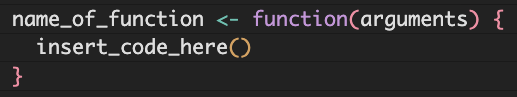
The general syntax of a function is like this:

name_of_function <- function(arguments) {
  insert_code_here()
}

You can pass multiple arguments to a function, but we are going to start simply with a function that takes one argument.

2.2 Functions with one argument

Here, I am writing a little function to do something simple, like calculate from millimeters to inches.

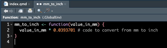
mm_to_inch <- function(value_in_mm) {
  value_in_mm * 0.0393701 # code to convert from mm to inch
}

Here, we would call value_in_mm our argument or parameter. Remember that this is a user-defined term, you could call this x, i, or really whatever you want. I like giving the arguments easy-to-read and easy-to-remember names.

Now that we’ve made a function, we can see it in our environment under the “Functions” header.

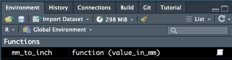
If we click on this item, we can see the details of the function.

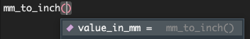
If we start typing our function, and put our cursor between the parentheses and press tab, we can also see some information about our function.

We can now pass arguments to our new function, here we will try passing 100 mm and see what that would be in inches.

mm_to_inch(value_in_mm = 100)

[1] 3.93701

Because our function only takes one argument, we can be less explicit and remove value_in_mm and get the same result.

mm_to_inch(100)

[1] 3.93701

We also might want to pass a whole column or vector to our function, which we can also do.

mm_to_inch(penguins$bill_length_mm)

  [1] 1.539371 1.555119 1.586615       NA 1.444883 1.547245 1.531497 1.543308
  [9] 1.342520 1.653544 1.488190 1.488190 1.618111 1.519686 1.362205 1.440946
 [17] 1.523623 1.673229 1.354331 1.811025 1.488190 1.484253 1.413387 1.503938
 [25] 1.527560 1.389765 1.598426 1.594489 1.492127 1.594489 1.555119 1.464568
 [33] 1.555119 1.610237 1.433072 1.543308 1.527560 1.661418 1.480316 1.566930
 [41] 1.437009 1.606300 1.417324 1.736221 1.456694 1.559056 1.618111 1.476379
 [49] 1.417324 1.665355 1.559056 1.578741 1.377953 1.653544 1.358268 1.629922
 [57] 1.535434 1.598426 1.437009 1.480316 1.405513 1.625985 1.480316 1.618111
 [65] 1.433072 1.637796 1.397639 1.618111 1.413387 1.645670 1.318898 1.562993
 [73] 1.559056 1.803151 1.397639 1.685040 1.610237 1.464568 1.425198 1.657481
 [81] 1.362205 1.688977 1.444883 1.381891 1.468505 1.625985 1.429135 1.452757
 [89] 1.507875 1.531497 1.405513 1.618111 1.338583 1.559056 1.425198 1.606300
 [97] 1.500001 1.586615 1.303150 1.700788 1.377953 1.614174 1.484253 1.488190
[105] 1.492127 1.562993 1.519686 1.503938 1.500001 1.700788 1.500001 1.795277
[113] 1.562993 1.661418 1.559056 1.681103 1.519686 1.468505 1.405513 1.618111
[121] 1.425198 1.484253 1.582678 1.629922 1.385828 1.598426 1.527560 1.633859
[129] 1.535434 1.736221 1.515749 1.696851 1.448820 1.476379 1.500001 1.618111
[137] 1.401576 1.582678 1.456694 1.562993 1.582678 1.598426 1.263780 1.602363
[145] 1.468505 1.535434 1.543308 1.440946 1.417324 1.488190 1.417324 1.633859
[153] 1.814962 1.968505 1.917324 1.968505 1.874017 1.830710 1.787403 1.838584
[161] 1.704725 1.842521 1.610237 1.929135 1.791340 1.905513 1.803151 1.940946
[169] 1.653544 1.937009 1.818899 1.917324 1.976379 1.775592 1.830710 1.822836
[177] 1.688977 1.814962 1.751969 1.881891 1.897639 1.968505 1.862206 1.685040
[185] 1.775592 2.346458 1.933072 1.905513 1.677166 1.748032 1.732284 1.917324
[193] 1.681103 1.952757 1.783466 1.952757 1.988190 1.716536 1.791340 1.988190
[201] 1.767717 1.779529 1.834647 1.909450 1.775592 1.972442 1.830710 1.771654
[209] 1.724410 1.791340 1.700788 1.984253 1.783466 1.818899 1.799214 2.137796
[217] 1.803151 1.960631 1.818899 1.948820 1.712599 1.996064 1.877954 1.826773
[225] 1.897639 1.830710 1.826773 1.913387 1.870080 2.011812 1.779529 1.779529
[233] 1.933072 2.066930 1.866143 1.968505 1.767717 2.000001 1.708662 2.019686
[241] 1.870080 2.051182 1.870080 2.055119 1.791340 1.948820 1.751969 2.000001
[249] 1.944883 1.846458 1.905513 2.011812 1.909450 2.200789 1.858269 1.933072
[257] 1.862206 1.842521 1.641733 2.102363 1.704725 1.893702 1.988190 1.960631
[265] 1.712599 2.027560 1.818899 2.169293 1.751969 1.921261 1.858269       NA
[273] 1.842521 1.984253 1.779529 1.964568 1.830710 1.968505 2.019686 1.787403
[281] 2.074804 1.779529 1.814962 2.019686 1.811025 2.019686 1.834647 2.035434
[289] 1.850395 2.047245 1.807088 1.988190 1.980316 2.283466 1.826773 1.937009
[297] 1.669292 1.909450 1.700788 1.992127 1.838584 2.047245 1.988190 1.948820
[305] 1.826773 2.078741 1.610237 2.133859 1.673229 2.007875 1.956694 1.870080
[313] 1.874017 2.047245 1.846458 2.106300 1.929135 1.818899 2.003938 1.791340
[321] 2.003938 2.000001 1.972442 1.929135 2.027560 1.960631 1.893702 2.023623
[329] 1.799214 1.996064 1.673229 2.055119 1.779529 1.940946 1.976379 1.795277
[337] 2.043308 1.842521 1.799214 2.196852 1.712599 1.952757 2.000001 1.976379

Instead of just printing this information, we might want to save it in our dataframe, which we can do by nesting our function within a mutate() function. Remember that mutate() works with the syntax new_column = function(existing_variables). Also remember that by default, new columns are added after the last column (and if you want to also reorder, you can do that with select()).

penguins |> 
  mutate(bill_length_inch = mm_to_inch(bill_length_mm))

# A tibble: 344 × 9
   species island    bill_length_mm bill_depth_mm flipper_length_mm body_mass_g
   <fct>   <fct>              <dbl>         <dbl>             <int>       <int>
 1 Adelie  Torgersen           39.1          18.7               181        3750
 2 Adelie  Torgersen           39.5          17.4               186        3800
 3 Adelie  Torgersen           40.3          18                 195        3250
 4 Adelie  Torgersen           NA            NA                  NA          NA
 5 Adelie  Torgersen           36.7          19.3               193        3450
 6 Adelie  Torgersen           39.3          20.6               190        3650
 7 Adelie  Torgersen           38.9          17.8               181        3625
 8 Adelie  Torgersen           39.2          19.6               195        4675
 9 Adelie  Torgersen           34.1          18.1               193        3475
10 Adelie  Torgersen           42            20.2               190        4250
# ℹ 334 more rows
# ℹ 3 more variables: sex <fct>, year <int>, bill_length_inch <dbl>

2.3 Embedding built in functions

We can also use other functions inside our function. For example, R does not by default have a function that calculates the coefficient of variation for a variable. We can write that ourselves though so it’s fine.

# calculate the coefficient of variation by 
# dividing the standard deviation by the mean
cv <- function(x) {
        (sd(x)/mean(x))
}

2.4 Functions with two arguments

We can also write functions that take more than one argument. Here is a simple example for calculating BMI, which is weight in kg divided by height in meters squared.

calculate_bmi <- function(weight_kg, height_cm) {
  weight_kg/(height_cm/100)^2
}

calculate_bmi(weight_kg = 80, height_cm = 180)

[1] 24.69136

If you provide your arguments in the order they are expected (here, weight_kg and then height_cm), then you don’t need to specify which is which. But, iif you want to give the arguments in a different order you need to be explicit.

# this is wrong
calculate_bmi(180, 80)

[1] 281.25

# this is better
calculate_bmi(height_cm = 180, weight_kg = 80)

[1] 24.69136

2.5 Functions with one argument practice

Write two functions that convert between degrees Fahrenheit and degrees Celsius and test to see if they work.

Need a hint?

°C = (°F - 32) × 5/9 or °F = (°C * 9/5) + 32

Click for the solution

# create a function to convert F to C
degF_to_degC <- function(deg_F) {
  (deg_F - 32) * (5/9)
}

# create a function to convert C to F
degC_to_degF <- function(deg_C) {
  (deg_C * (9/5)) + 32
}

degF_to_degC(deg_F = 32)

[1] 0

degF_to_degC(deg_F = 100)

[1] 37.77778

degC_to_degF(deg_C = 0)

[1] 32

degC_to_degF(deg_C = -40)

[1] -40

2.6 Plotting functions

Now that we are a little comfortable with writing functions, we can make ones that are a little more complicated.

We can also write a function to make our plot.

species_bill_plotting <- function(focal_species) {
    penguins |> 
    filter(species == focal_species) |> 
    drop_na() |> 
    ggplot(aes(x = bill_length_mm, y = bill_depth_mm, color = sex)) +
    geom_point() + 
    geom_smooth(method = "lm", # use a linear model
                se = FALSE) + # turn off confidence interval
    scale_color_brewer(palette = "Dark2") +
    labs(title = focal_species, # put the species name as the title
         x = "Bill length (mm)",
         y = "Bill depth (mm)",
         color = "Sex", 
         caption = "Data collected from LTER, Antarctica") + 
    theme_classic() 
}

Then, we can pass our argument to the plot, here, the name of the species we want to plot. This is a useful tool for making many plots with the same structure.

species_bill_plotting("Adelie")

`geom_smooth()` using formula = 'y ~ x'

We can then pass this function in a for loop with some simpler looking code (because the bulk of it is elsewhere).

penguin_species <- unique(penguins$species)

for (focal_species in penguin_species) {
  # pass each focal species to the species_bill_plotting function
  plot <- species_bill_plotting(focal_species)

# save the plots
  filename <- glue("figs/{focal_species}_bill-dimensions.png") # create filename
  ggsave(filename, plot) # save the plot to file
}

Saving 7 x 5 in image
`geom_smooth()` using formula = 'y ~ x'
Saving 7 x 5 in image
`geom_smooth()` using formula = 'y ~ x'
Saving 7 x 5 in image
`geom_smooth()` using formula = 'y ~ x'

2.7 Writing plotting functions practice

Write a function to make a series of boxplots that show the difference in body_mass_g between male and female penguins by species. Feed one species to your function to check if it works (you don’t need to iterate with it yet).

Need a hint?

Check back to our example where we used a for loop to see how to make this plot.

Click for the solution

# create the function
body_mass_by_sex_plotting <- function(focal_species) {
    penguins |> 
    filter(species == focal_species) |> 
    drop_na(sex, body_mass_g) |> 
    ggplot(aes(x = sex, y = body_mass_g, color = sex)) +
      geom_boxplot() +
      theme_minimal() +
      scale_color_brewer(palette = "Dark2") +
      theme(legend.position = "none") + # don't need one bc duplicative with x-axis
      labs(x = "Sex",
        y = "Body mass (grams)",
        title = focal_species)
}

# apply the function to Adelie penguins
body_mass_by_sex_plotting("Adelie")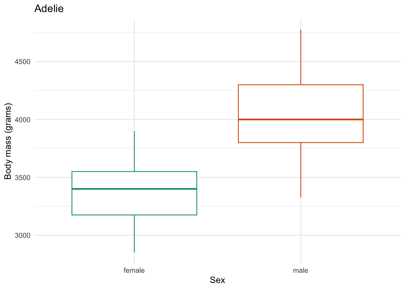

3 Iteration with `purrr:map`

To simplify our code, we could replace our for loop with one of the tidyverse:purrr functions intended for functional program that being with map*().

But before we do this, we need to learn a little bit about lists.

3.1 About lists

A list is a new data structure for Code Club. A list can contain other data structures, like data frames, vectors or others, within it.

To see what a list looks like, we will look under the hood at the object that comprises a ggplot plot. We have one in our environment called plot so let’s look at that.

View(plot)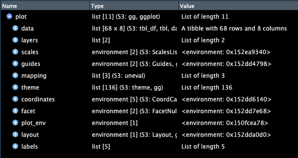

We can see that in this case, plot is a list which contains 11 objects, many of which also contain sub-objects. For example, data is a dataframe that. contains the data underlying our plot. It is a tibble type of dataframe with 68 rows and 8 columns.

If I want to access that first item in the list, I can do that in a few different ways.

I can use the dollar sign operator $ to extract parts of the list

plot$data

# A tibble: 68 × 8
   species   island bill_length_mm bill_depth_mm flipper_length_mm body_mass_g
   <fct>     <fct>           <dbl>         <dbl>             <int>       <int>
 1 Chinstrap Dream            46.5          17.9               192        3500
 2 Chinstrap Dream            50            19.5               196        3900
 3 Chinstrap Dream            51.3          19.2               193        3650
 4 Chinstrap Dream            45.4          18.7               188        3525
 5 Chinstrap Dream            52.7          19.8               197        3725
 6 Chinstrap Dream            45.2          17.8               198        3950
 7 Chinstrap Dream            46.1          18.2               178        3250
 8 Chinstrap Dream            51.3          18.2               197        3750
 9 Chinstrap Dream            46            18.9               195        4150
10 Chinstrap Dream            51.3          19.9               198        3700
# ℹ 58 more rows
# ℹ 2 more variables: sex <fct>, year <int>

Or, I can use indexing to extract out the first item in our list.

plot[1]

$data
# A tibble: 68 × 8
   species   island bill_length_mm bill_depth_mm flipper_length_mm body_mass_g
   <fct>     <fct>           <dbl>         <dbl>             <int>       <int>
 1 Chinstrap Dream            46.5          17.9               192        3500
 2 Chinstrap Dream            50            19.5               196        3900
 3 Chinstrap Dream            51.3          19.2               193        3650
 4 Chinstrap Dream            45.4          18.7               188        3525
 5 Chinstrap Dream            52.7          19.8               197        3725
 6 Chinstrap Dream            45.2          17.8               198        3950
 7 Chinstrap Dream            46.1          18.2               178        3250
 8 Chinstrap Dream            51.3          18.2               197        3750
 9 Chinstrap Dream            46            18.9               195        4150
10 Chinstrap Dream            51.3          19.9               198        3700
# ℹ 58 more rows
# ℹ 2 more variables: sex <fct>, year <int>

3.2 `map()`

The simplest of the functions in purrr is map(), which applies a function over each element of a vector, and returns a list. There are some basics we will have to go over for this to make sense.

The map(), we provide a vector/list to iterate over, and a function, like this:

map(.x = 1:5, # our vector to apply our function over
    function(x) x + 1) # what the function is

[[1]]
[1] 2

[[2]]
[1] 3

[[3]]
[1] 4

[[4]]
[1] 5

[[5]]
[1] 6

Now let’s get back to the function we wrote to make our plots - instead of incorporating this into a for loop, we can apply it within map() like this:

map(penguin_species, # vector to iterate over
    species_bill_plotting) # function to use

[[1]]

`geom_smooth()` using formula = 'y ~ x'


[[2]]

`geom_smooth()` using formula = 'y ~ x'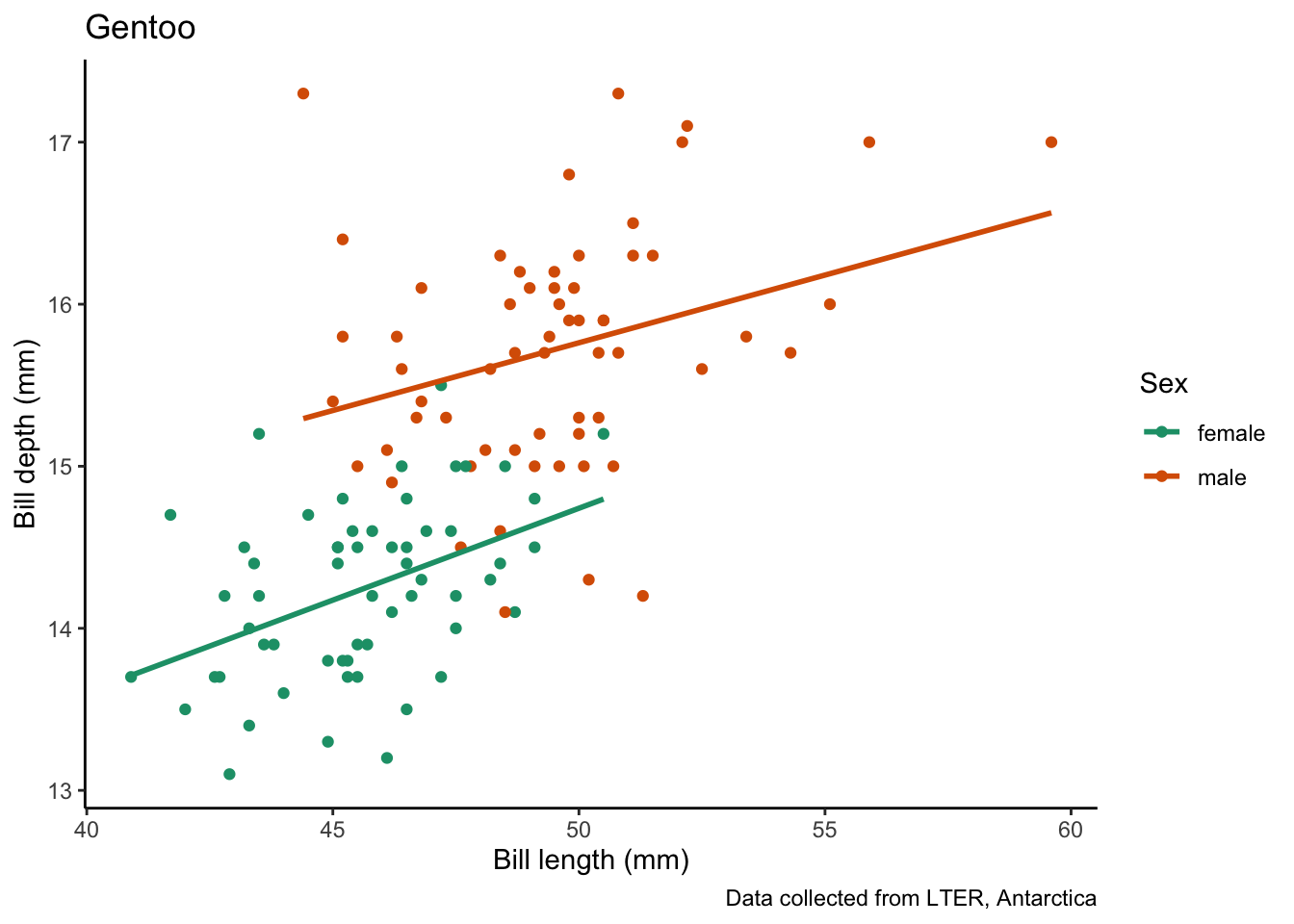


[[3]]

`geom_smooth()` using formula = 'y ~ x'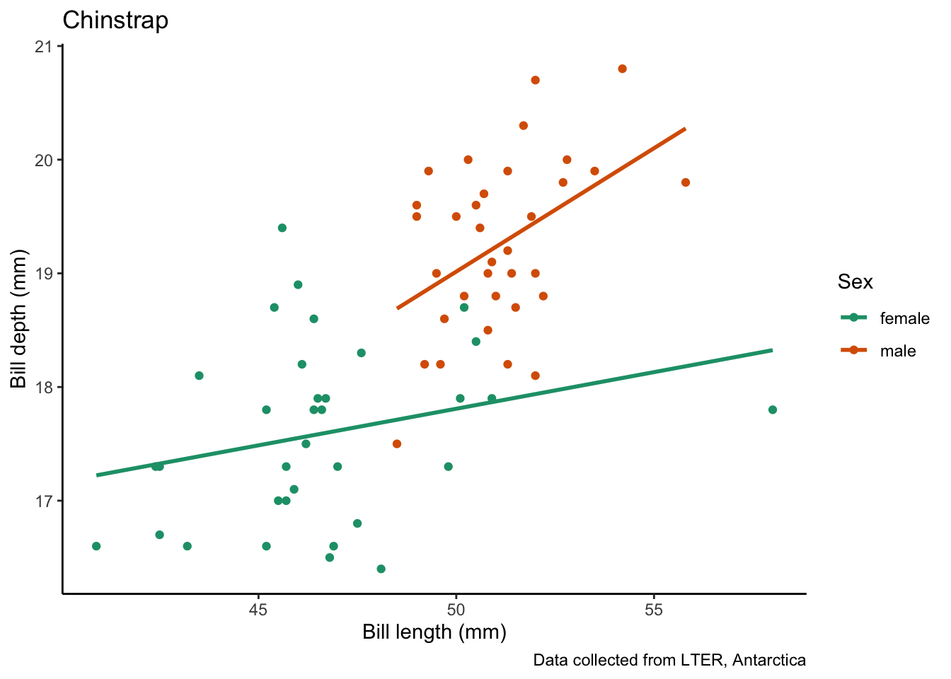

Wow that was simple!

We could also incorporate both the printing and saving of the plot into one function like this:

species_bill_plotting_saving <- function(focal_species) {
  
# create plot and assign it to something 
  plot_via_function <- penguins |> 
    filter(species == focal_species) |> 
    drop_na() |> 
    ggplot(aes(x = bill_length_mm, y = bill_depth_mm, color = sex)) +
    geom_point() + 
    geom_smooth(method = "lm", # use a linear model
                se = FALSE) + # turn off confidence interval
    scale_color_brewer(palette = "Dark2") +
    labs(title = focal_species, # put the species name as the title
         x = "Bill length (mm)",
         y = "Bill depth (mm)",
         color = "Sex", 
         caption = "Data collected from LTER, Antarctica") + 
    theme_classic() 
  
# print
  print(plot_via_function)
  
# save
  filename <- glue("figs/{focal_species}_bill-dimensions-via-function.png") # choose filename
  ggsave(filename, plot_via_function) # save the plot to file
}

Then, this code will:

Generate your plots
Print those plots for you to view in RStudio
Save those plots in a directory called figs in your working directory

map(penguin_species, # vector to iterate over
    species_bill_plotting_saving) # function to apply

`geom_smooth()` using formula = 'y ~ x'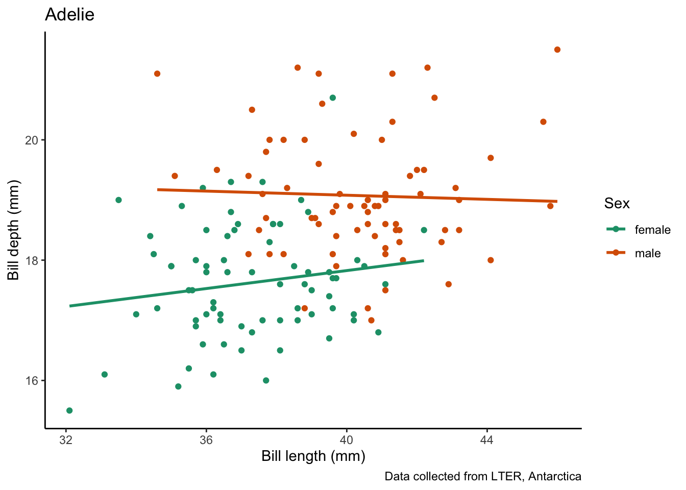

Saving 7 x 5 in image
`geom_smooth()` using formula = 'y ~ x'
`geom_smooth()` using formula = 'y ~ x'

Saving 7 x 5 in image
`geom_smooth()` using formula = 'y ~ x'
`geom_smooth()` using formula = 'y ~ x'

Saving 7 x 5 in image
`geom_smooth()` using formula = 'y ~ x'

[[1]]
figs/Adelie_bill-dimensions-via-function.png

[[2]]
figs/Gentoo_bill-dimensions-via-function.png

[[3]]
figs/Chinstrap_bill-dimensions-via-function.png

3.3 Functions with more arguments practice

Try applying your function you made to create a series of boxplots for body mass by sex over each of the penguin species, though edit it so it both prints and saves your plots.

Need a hint?

Here is my hint

Click for the solution

Edit the function to include printing and saving.

species_body_mass_sex_plotting_saving <- function(focal_species) {
  my_plot <- penguins |> 
    filter(species == focal_species) |> 
    drop_na(sex, body_mass_g) |> 
    ggplot(aes(x = sex, y = body_mass_g, color = sex)) +
      geom_boxplot() +
      theme_minimal() +
      scale_color_brewer(palette = "Dark2") +
      theme(legend.position = "none") + # don't need one bc duplicative with x-axis
      labs(x = "Sex",
        y = "Body mass (grams)",
        title = focal_species)

# print
  print(my_plot)
  
# save
  filename <- glue("figs/{focal_species}_body-mass-by-sex.png") # choose filename
  ggsave(filename, my_plot) # save the plot to file
}

Apply the function across the species

map(penguin_species, # what to iterate over
    species_body_mass_sex_plotting_saving) # the function to iterate with

Saving 7 x 5 in image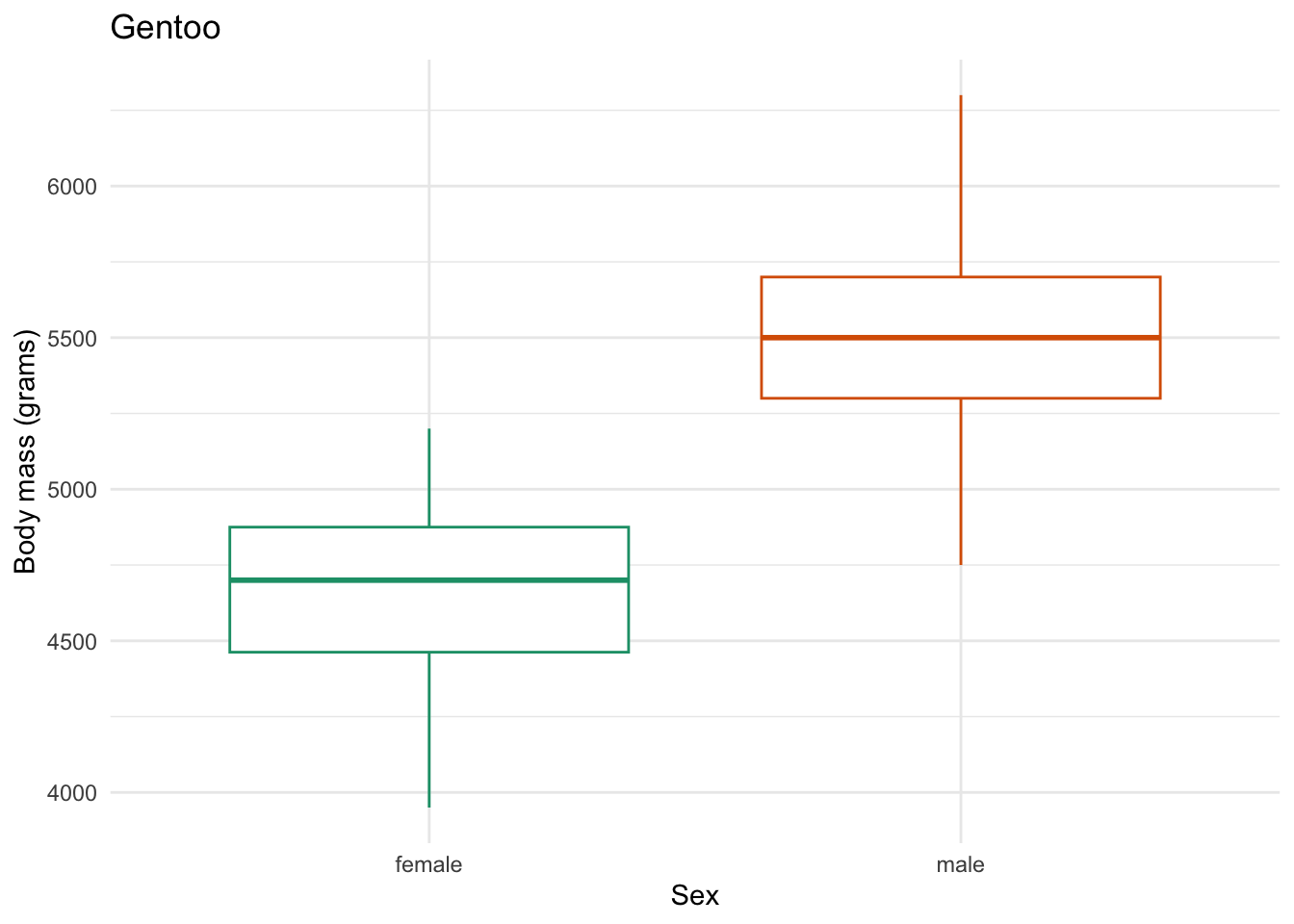

Saving 7 x 5 in image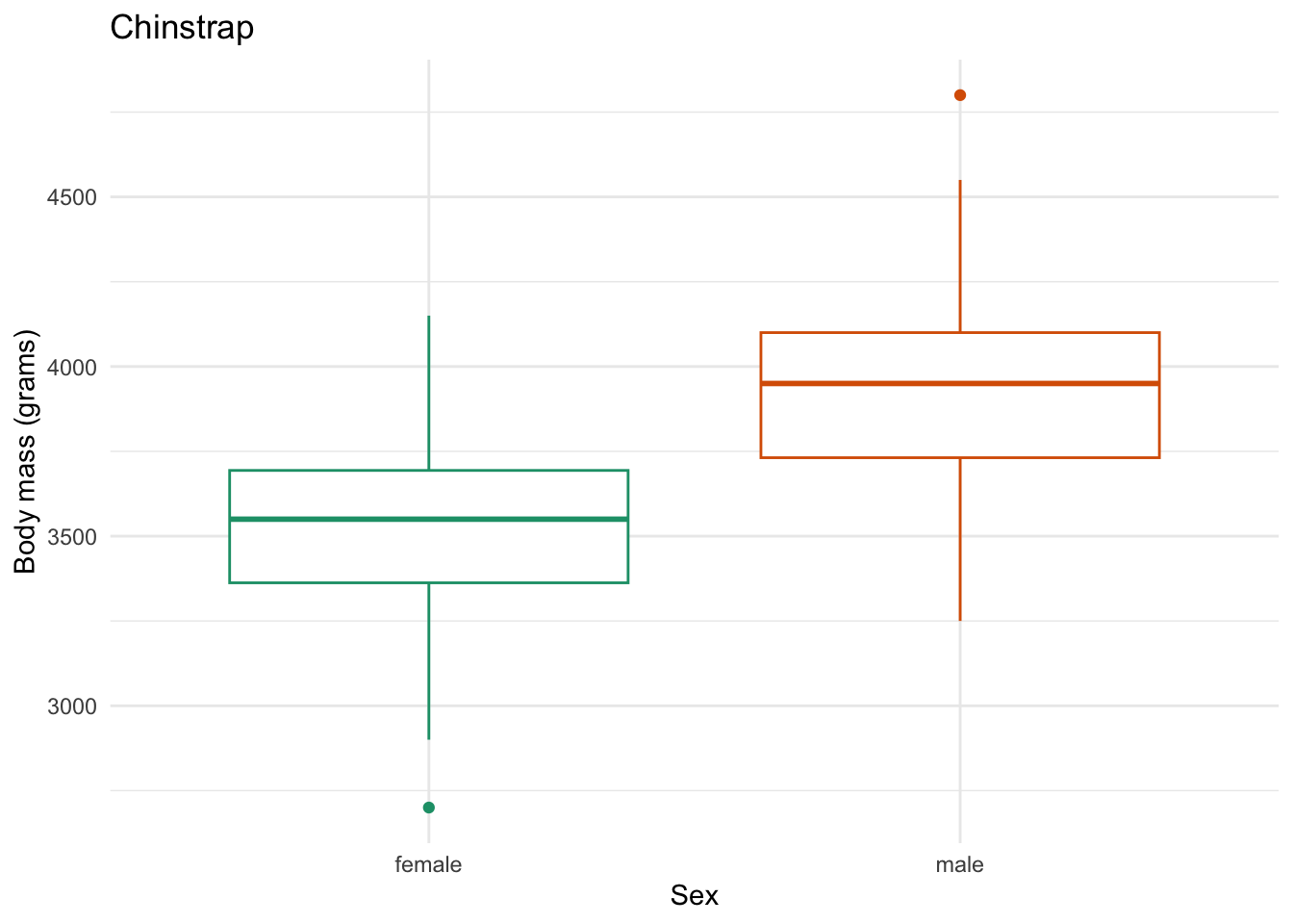

Saving 7 x 5 in image

[[1]]
figs/Adelie_body-mass-by-sex.png

[[2]]
figs/Gentoo_body-mass-by-sex.png

[[3]]
figs/Chinstrap_body-mass-by-sex.png

1 Introduction

2 Writing functions

2.1 General syntax

2.2 Functions with one argument

2.3 Embedding built in functions

2.4 Functions with two arguments

2.5 Functions with one argument practice

2.6 Plotting functions

2.7 Writing plotting functions practice

3 Iteration with purrr:map

3.1 About lists

3.2 map()

3.3 Functions with more arguments practice

3 Iteration with `purrr:map`

3.2 `map()`