Data Wrangling 3: Counting and Summarizing Data by Group

r-basics

tidyverse

Author

Jelmer Poelstra

Published

September 16, 2024

1 Introduction

Recap of the past two weeks

In the past two weeks, we’ve been learning about the following functions from the dplyr package, a central workhorse of the tidyverse ecosystem, to manipulate data in data frames:

filter() to pick rows (which typically represent observations/samples/individuals)
select() to pick columns (which typically represent variables/properties)
arrange() to sort data frame rows
mutate() to add and manipulate data frame columns

Learning objectives for today

Our main focus is another very useful dplyr function: summarize() to compute summaries across rows, typically across groups of rows.
We will start with an introduction to a new dataset, the count() function, and dealing with missing data.
If we manage to get to it, we will also learn about the slice_() family of functions, to pick rows in a different manner than with filter().

Setting up

Load the tidyverse meta-package:

library(tidyverse)

── Attaching core tidyverse packages ──────────────────────── tidyverse 2.0.0 ──
✔ dplyr     1.1.4     ✔ readr     2.1.5
✔ forcats   1.0.0     ✔ stringr   1.5.1
✔ ggplot2   3.5.1     ✔ tibble    3.2.1
✔ lubridate 1.9.3     ✔ tidyr     1.3.1
✔ purrr     1.0.2     
── Conflicts ────────────────────────────────────────── tidyverse_conflicts() ──
✖ dplyr::filter() masks stats::filter()
✖ dplyr::lag()    masks stats::lag()
ℹ Use the conflicted package (<http://conflicted.r-lib.org/>) to force all conflicts to become errors

Still need to install the tidyverse? Click here for instructions

install.packages("tidyverse")

2 A penguins dataset

The data set we will use today is from the palmerpenguins package, which contains a data set on 🐧 collected by Dr. Kristen Gorman at the Palmer Station Antarctica.

It is a nice, relatively simple data set to practice data exploration and visualization in R.

Installing and loading the package

We’ll have to install that package first, which should be quick:

install.packages("palmerpenguins")

Now we’re ready to load the package:

library(palmerpenguins)

Taking a look at the data set

Once you’ve loaded the palmerpenguins package, you will have a data frame called penguins at your disposal — let’s take a look:

penguins

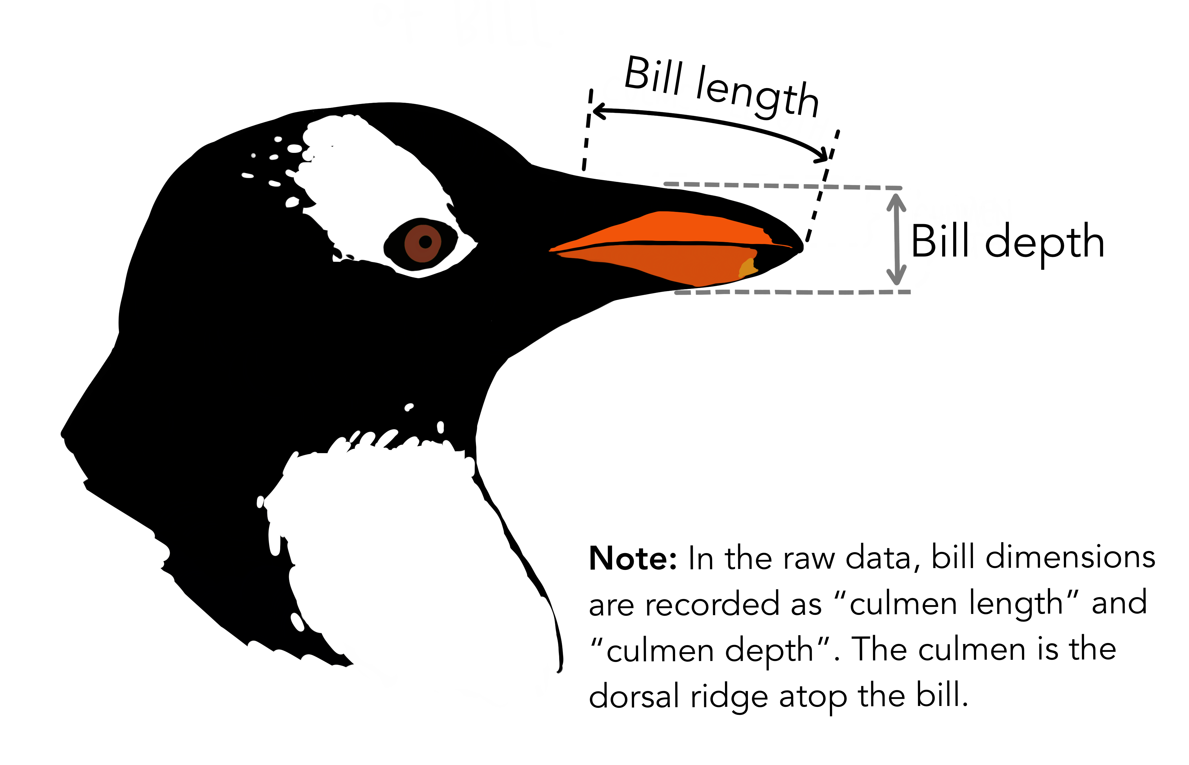
In this data set, each row represents an individual penguin for which we know the species, sex, island of origin, and for which, across several years, we have a set of size measurements:

Bill length in mm (bill_length_mm column)
Bill depth in mm (bill_depth_mm column)
Flipper length in mm (flipper_length_mm column)
Body mass in grams (body_mass_g column)

Here’s a visual for what the two bill measurements represent:

3 Exploring data with the `count()` function

To orient yourself a bit more to this dataset, you may want to see, for example, how many species and how many islands are in it, and how frequently each occur.

In other words, we may want to produce a few “count tables”, which is a common part of Exploratory Data Analysis (EDA). We can do this with the dplyr function count():

penguins |> count(species)

# A tibble: 3 × 2
  species       n
  <fct>     <int>
1 Adelie      152
2 Chinstrap    68
3 Gentoo      124

penguins |> count(island)

# A tibble: 3 × 2
  island        n
  <fct>     <int>
1 Biscoe      168
2 Dream       124
3 Torgersen    52

OK, so we have penguins that belong to 3 different species occur on 3 different islands. Which species occur on which islands? We can answer this with count() simply by specifying both columns:

penguins |> count(species, island)

# A tibble: 5 × 3
  species   island        n
  <fct>     <fct>     <int>
1 Adelie    Biscoe       44
2 Adelie    Dream        56
3 Adelie    Torgersen    52
4 Chinstrap Dream        68
5 Gentoo    Biscoe      124

Why are not all possible combinations of species and island shown here?

Some species do not appear to occur on (or at least haven’t been sampled on) certain islands. These zero-counts are not show, or “dropped, by default.

To show zero-count combinations, add .drop = FALSE:

penguins |> count(species, island, .drop = FALSE)

# A tibble: 9 × 3
  species   island        n
  <fct>     <fct>     <int>
1 Adelie    Biscoe       44
2 Adelie    Dream        56
3 Adelie    Torgersen    52
4 Chinstrap Biscoe        0
5 Chinstrap Dream        68
6 Chinstrap Torgersen     0
7 Gentoo    Biscoe      124
8 Gentoo    Dream         0
9 Gentoo    Torgersen     0

Side note: Base R’s table() function (Click to expand)

Also worth mentioning is the base R table() function, which is similar to count(). While its output format is unwieldy for follow-up analyses, you may prefer its formatting especially when wanting to glance at a 2-way count table to see patterns:

table(penguins$species, penguins$island)

           
            Biscoe Dream Torgersen
  Adelie        44    56        52
  Chinstrap      0    68         0
  Gentoo       124     0         0

Additionally, as a dplyr function, count() only works with data frames. You may sometimes need to create a count table for a vector, and table() can do that:

species_vector <- penguins$species
table(species_vector)

species_vector
   Adelie Chinstrap    Gentoo 
      152        68       124

4 Missing data

Let’s compute the mean bill length across all penguins: we can do so by running the mean() function on the bill length column from the penguins data frame, which we can extract using the base R $ notation, penguins$bill_length_mm:

mean(penguins$bill_length_mm)

[1] NA

What does NA mean and why are we getting this?

NA means “not any” and is R’s way of representing missing data. When a computation in R returns NA, this means that some of the values used must themselves have been NA. In other words, one or more of the values in the bill_length_mm columns are NA: perhaps the penguin in question got away before its bill was measured.

We can overcome this issue, and compute the mean among the non-missing bill length values, by setting the argument na.rm (“NA-remove”) to TRUE – and note that this argument is available in many functions in R:

mean(penguins$bill_length_mm, na.rm = TRUE)

[1] 43.92193

Let’s find the penguins with a missing bill length measurement using filter() in combination with the is.na() function, which tests whether a value is NA or not:

penguins |>
  filter(is.na(bill_length_mm))

5 Exercises I

5.1 `count()`

A) Use count() to get the number of penguins for each combination of species, year and sex.

Solution (click here)

penguins |> count(species, year, sex)

# A tibble: 22 × 4
   species    year sex        n
   <fct>     <int> <fct>  <int>
 1 Adelie     2007 female    22
 2 Adelie     2007 male      22
 3 Adelie     2007 <NA>       6
 4 Adelie     2008 female    25
 5 Adelie     2008 male      25
 6 Adelie     2009 female    26
 7 Adelie     2009 male      26
 8 Chinstrap  2007 female    13
 9 Chinstrap  2007 male      13
10 Chinstrap  2008 female     9
# ℹ 12 more rows

B) What is the least common combination of species and sex for penguins weighing less than 4,000 grams?

Hint (click here)

You’ll have to filter() first.

Solution (click here)

The least common combination among such light-weight penguins is female Gentoo, of which there is only 1. Or you may also argue that the answer should be male Gentoo, of which there are none.

In the code below, I’m sorting the dataframe by the count (column n), so we’ll see the least common combinations at the top:

penguins |>
  filter(body_mass_g < 4000) |> 
  count(species, sex, .drop = FALSE) |>
  arrange(n)

# A tibble: 7 × 3
  species   sex        n
  <fct>     <fct>  <int>
1 Gentoo    male       0
2 Gentoo    female     1
3 Adelie    <NA>       4
4 Chinstrap male      19
5 Chinstrap female    33
6 Adelie    male      35
7 Adelie    female    73

P.S.: count() does have a sort argument so you can omit the separate call to arrange(), though note that it can only sort descendingly:

penguins |>
  filter(body_mass_g < 4000) |> 
  count(species, sex, .drop = FALSE, sort = TRUE)

# A tibble: 7 × 3
  species   sex        n
  <fct>     <fct>  <int>
1 Adelie    female    73
2 Adelie    male      35
3 Chinstrap female    33
4 Chinstrap male      19
5 Adelie    <NA>       4
6 Gentoo    female     1
7 Gentoo    male       0

5.2 Removing rows with missing data

For the sake of convenience, we will here remove these two penguins that don’t seem to have had any measurements taken¹.

A) Do so by storing the output of an appropriate filter() operation in a new data frame penguins_noNA.

Hint (click here)

The code will be very similar to our is.na filtering operation above, except that you should negate this using a !: this will instead keep rows that are not NA.

Solution (click here)

penguins_noNA <- penguins |>
  filter(!is.na(bill_length_mm))

B) Check how many penguins (rows) were removed.

Solution (click here)

2 rows should have been removed.

There are many ways to check this! You can simply look for these objects in the Environment pane, print them to screen, or use the nrow() function:

nrow(penguins)

[1] 344

nrow(penguins_noNA)

[1] 342

nrow(penguins) - nrow(penguins_noNA)

[1] 2

Side note: Checking and removing all columns with missing data (Click to expand)

You can see rows with missing data in any column, regardless of how many there are in total, using the if_any() helper function of filter():

Its first argument is a column selection (here, everything() will select all columns),
Its second argument is the name of a function to run for each column (here, is.na)
Rows for which the function returns TRUE in any (hence “if_any()”) of the will be kept.

penguins |>
  filter(if_any(everything(), is.na))

It looks like besides the 2 rows with missing measurements, there are also 9 rows where the sex of the penguins is missing (on the website, click the right arrow to see that column).

Removing all rows with missing data could be done by adding a ! to the above code, but there is also a drop_na() convenience function available:

penguins_noNA2 <- penguins |>
  drop_na()

Let’s check the numbers of rows in the different data frames:

nrow(penguins)         # The original data frame

[1] 344

nrow(penguins_noNA)    # Without the 2 penguins with missing measurements

[1] 342

nrow(penguins_noNA2)   # Without all rows with missing data

[1] 333

6 The `summarize()` function

The summarize() function from the dplyr package can compute across-row data summaries. As a first example, here’s how you can compute the overall mean bill length with this function:

penguins_noNA |>
  summarize(mean(bill_length_mm))

# A tibble: 1 × 1
  `mean(bill_length_mm)`
                   <dbl>
1                   43.9

(Note that we are now using penguins_noNA, which you created in the exercise above, and we will continue to do so during the rest of the session.)

As you can see, this function has quite a different output from the dplyr functions we’d seen so far. All of those returned a manipulated version of our original dataframe, whereas summarize() returns a “completely new” dataframe with a summary of the original data.

Note that the default summary column above is quite unwieldy, so we’ll typically want to provide a column name for it ourselves:

penguins_noNA |>
  summarize(bill_len_mean = mean(bill_length_mm))

# A tibble: 1 × 1
  bill_len_mean
          <dbl>
1          43.9

Also, summarizing across all rows at once with summarize(), like we just did, is much more verbose than the simple “base R” solution we saw earlier (mean(penguins_noNA$bill_length_mm)). Are we sure this function is useful?

Summarizing by group

The real power of summarize() comes with its ability to easily compute group-wise summaries. For example, simply by adding .by = species, it will calculate the mean bill length separately for each species:

penguins_noNA |>
  summarize(bill_len_mean = mean(bill_length_mm), .by = species)

# A tibble: 3 × 2
  species   bill_len_mean
  <fct>             <dbl>
1 Adelie             38.8
2 Gentoo             47.5
3 Chinstrap          48.8

Nice! We can also compute multiple summarized variables — and use summarizing functions other than mean():

penguins_noNA |>
  summarize(bill_len_mean = mean(bill_length_mm),
            bill_len_max = max(bill_length_mm),
            bill_len_min = min(bill_length_mm),
            .by = species)

# A tibble: 3 × 4
  species   bill_len_mean bill_len_max bill_len_min
  <fct>             <dbl>        <dbl>        <dbl>
1 Adelie             38.8         46           32.1
2 Gentoo             47.5         59.6         40.9
3 Chinstrap          48.8         58           40.9

Including group counts

A handy helper function related to the count() function we used above is n(), which will compute the number of rows for each group (i.e. the group sizes, which can be good to know, for example so you don’t make unfounded conclusions based on really small sample sizes):

penguins_noNA |>
  summarize(bill_depth_mean = mean(bill_depth_mm),
            n_penguins = n(),
            .by = species)

# A tibble: 3 × 3
  species   bill_depth_mean n_penguins
  <fct>               <dbl>      <int>
1 Adelie               18.3        151
2 Gentoo               15.0        123
3 Chinstrap            18.4         68

Common summary statistic functions

Here is an overview of the most commonly used functions to compute summaries:

mean() & median()
min() & max()
sum()
sd(): standard deviation
IQR(): interquartile range
n(): counts the number of rows (observations)
n_distinct(): counts the number of distinct (unique) values

Two final comments about summarize():

You can also ask summarize() to compute summaries by multiple columns, which will return separate summaries for each combination of the involved variables — we’ll see this in the exercises.
This may be obvious, but whatever column you are computing summaries by (using .by) should be a categorical variable. In our diamond examples, we’re only using columns that are factors, but “regular” character columns will work just fine as well.

Side note: group_by() (Click to expand)

The “classic” way of using summarize() with multiple groups is by preceding it with a group_by() call — e.g., the code below is equivalent to our last example above:

penguins_noNA |>
  group_by(species) |> 
  summarize(bill_depth_mean = mean(bill_depth_mm),
            n_penguins = n())

# A tibble: 3 × 3
  species   bill_depth_mean n_penguins
  <fct>               <dbl>      <int>
1 Adelie               18.3        151
2 Chinstrap            18.4         68
3 Gentoo               15.0        123

The .by argument to summarize() (and other functions!) is a rather recent addition, but I prefer it over group_by():

It is simpler, a bit less typing, and makes the summarize() call self-contained
When grouping by multiple columns, group_by() has some odd, unhelpful behavior where it keeps some of the groupings, such that you likely need an ungroup() call as well.

7 Exercises II

7.1 Means across variables

Compute the per-species means for all 4 size-related variables.

Do all these variables co-vary, such that, for example, one species is the largest for each measurement?

Solution (click here)

penguins_noNA |>
  summarize(bill_len = mean(bill_length_mm),
            bill_dep = mean(bill_depth_mm),
            flip_len = mean(flipper_length_mm),
            body_mass = mean(body_mass_g),
            .by = species)

# A tibble: 3 × 5
  species   bill_len bill_dep flip_len body_mass
  <fct>        <dbl>    <dbl>    <dbl>     <dbl>
1 Adelie        38.8     18.3     190.     3701.
2 Gentoo        47.5     15.0     217.     5076.
3 Chinstrap     48.8     18.4     196.     3733.

The variables seem to largely co-vary across species, but bill depth stands out: the large Gentoo penguins have less deep bills than the other two species.

7.2 Summaries across multiple groups

For Adelie penguins only, find the combination of island and year on which the lightest penguins were found, on average.

For this, you’ll have to group by both abovementioned columns. See if you can figure this out by yourself first, but check out the grouping hint below if you can’t get that part to work.

Grouping hint (click here)

.by = c(island, year) will group by these 2 columns at once.

More hints (click here)

filter() before you summarize to only keep Adelie penguins.
arrange() after you summarize to see the lowest mean weights at the top.

Solution (click here)

penguins_noNA |>
  filter(species == "Adelie") |> 
  summarize(mass_mean = mean(body_mass_g),
            .by = c(island, year)) |>
  arrange(mass_mean)

# A tibble: 9 × 3
  island     year mass_mean
  <fct>     <int>     <dbl>
1 Torgersen  2009     3489.
2 Biscoe     2007     3620 
3 Biscoe     2008     3628.
4 Dream      2009     3651.
5 Dream      2007     3671.
6 Dream      2008     3756.
7 Torgersen  2007     3763.
8 Torgersen  2008     3856.
9 Biscoe     2009     3858.

8 Bonus: The `slice_` functions

Like the filter() function, functions in the slice_ family select specific rows, but have some different functionality that’s quite handy — especially in combination with grouping.

Let’s say we wanted to only get, for each species, the lightest penguin. We can do this pretty easily with the slice_max() function, which will return the row(s) with the lowest value for a specified variable:

penguins_noNA |>
  slice_min(body_mass_g, by = species)

# A tibble: 4 × 8
  species   island bill_length_mm bill_depth_mm flipper_length_mm body_mass_g
  <fct>     <fct>           <dbl>         <dbl>             <int>       <int>
1 Adelie    Biscoe           36.5          16.6               181        2850
2 Adelie    Biscoe           36.4          17.1               184        2850
3 Gentoo    Biscoe           42.7          13.7               208        3950
4 Chinstrap Dream            46.9          16.6               192        2700
# ℹ 2 more variables: sex <fct>, year <int>

Why are we getting more than one penguin per species in some cases? (Click to see the answer)

Because of ties in the body_mass_g value. (We’ll get back to this in the next set of exercises.)

You can get more than just the single highest (slice_max()) / lowest (slice_min()) value per group with the n= argument, and can get a specific proportion of rows with prop=:

# Get the 3 penguins with the longest flippers for each year:
penguins_noNA |>
  slice_max(flipper_length_mm, by = year, n = 3)

# A tibble: 10 × 8
   species island bill_length_mm bill_depth_mm flipper_length_mm body_mass_g
   <fct>   <fct>           <dbl>         <dbl>             <int>       <int>
 1 Gentoo  Biscoe           50            16.3               230        5700
 2 Gentoo  Biscoe           59.6          17                 230        6050
 3 Gentoo  Biscoe           48.7          15.1               222        5350
 4 Gentoo  Biscoe           47.3          15.3               222        5250
 5 Gentoo  Biscoe           54.3          15.7               231        5650
 6 Gentoo  Biscoe           49.8          16.8               230        5700
 7 Gentoo  Biscoe           48.6          16                 230        5800
 8 Gentoo  Biscoe           52.1          17                 230        5550
 9 Gentoo  Biscoe           51.5          16.3               230        5500
10 Gentoo  Biscoe           55.1          16                 230        5850
# ℹ 2 more variables: sex <fct>, year <int>

# Get the 2% narrowest-billed penguins for each sex
penguins_noNA |>
  slice_min(bill_depth_mm, by = sex, prop = 0.02)

# A tibble: 6 × 8
  species island bill_length_mm bill_depth_mm flipper_length_mm body_mass_g
  <fct>   <fct>           <dbl>         <dbl>             <int>       <int>
1 Gentoo  Biscoe           48.5          14.1               220        5300
2 Gentoo  Biscoe           51.3          14.2               218        5300
3 Gentoo  Biscoe           50.2          14.3               218        5700
4 Gentoo  Biscoe           42.9          13.1               215        5000
5 Gentoo  Biscoe           46.1          13.2               211        4500
6 Gentoo  Biscoe           44.9          13.3               213        5100
# ℹ 2 more variables: sex <fct>, year <int>

The full set of slice_ functions

slice_head(n = 1) takes the first row.
slice_tail(n = 1) takes the last row
slice_min(x, n = 1) takes the row with the smallest value in column x.
slice_max(x, n = 1) takes the row with the largest value in column x.
slice_sample(n = 1) takes one random row.
slice(15) takes the 15th row.

9 Exercises III

9.1 No ties, please

Above, when we first used slice_min(), we got multiple rows for some groups. Check out the help for this function (?slice_min) and get it to print only one row per group, even in the case of ties.

Solution (click here)

The with_ties argument controls this. The default is TRUE (do include ties), so we want to set it to FALSE (don’t include ties):

penguins_noNA |>
  slice_min(body_mass_g, by = species, with_ties = FALSE)

# A tibble: 3 × 8
  species   island bill_length_mm bill_depth_mm flipper_length_mm body_mass_g
  <fct>     <fct>           <dbl>         <dbl>             <int>       <int>
1 Adelie    Biscoe           36.5          16.6               181        2850
2 Gentoo    Biscoe           42.7          13.7               208        3950
3 Chinstrap Dream            46.9          16.6               192        2700
# ℹ 2 more variables: sex <fct>, year <int>

9.2 Random penguins

Use slice_sample() to get 5 random penguins for each combination of year and island.

Solution (click here)

penguins_noNA |>
  slice_sample(n = 5, by = c(year, island))

# A tibble: 45 × 8
   species island    bill_length_mm bill_depth_mm flipper_length_mm body_mass_g
   <fct>   <fct>              <dbl>         <dbl>             <int>       <int>
 1 Adelie  Torgersen           36.6          17.8               185        3700
 2 Adelie  Torgersen           40.3          18                 195        3250
 3 Adelie  Torgersen           42.5          20.7               197        4500
 4 Adelie  Torgersen           38.9          17.8               181        3625
 5 Adelie  Torgersen           46            21.5               194        4200
 6 Gentoo  Biscoe              50.2          14.3               218        5700
 7 Gentoo  Biscoe              42            13.5               210        4150
 8 Gentoo  Biscoe              48.7          15.1               222        5350
 9 Gentoo  Biscoe              45.1          14.5               207        5050
10 Gentoo  Biscoe              46.1          13.2               211        4500
# ℹ 35 more rows
# ℹ 2 more variables: sex <fct>, year <int>

Footnotes

Removing rows with NAs may be appropriate for your own data too, but this will depend on the context!↩︎

1 Introduction

Recap of the past two weeks

Learning objectives for today

Setting up

2 A penguins dataset

Installing and loading the package

Taking a look at the data set

3 Exploring data with the count() function

4 Missing data

5 Exercises I

5.1 count()

5.2 Removing rows with missing data

6 The summarize() function

Summarizing by group

Including group counts

Common summary statistic functions

7 Exercises II

7.1 Means across variables

7.2 Summaries across multiple groups

8 Bonus: The slice_ functions

9 Exercises III

9.1 No ties, please

9.2 Random penguins

Footnotes

3 Exploring data with the `count()` function

5.1 `count()`

6 The `summarize()` function

8 Bonus: The `slice_` functions