Data wrangling with dplyr

Authors

Affiliation

Software Carpentry

Jelmer Poelstra

CFAES Bioinformatics Core, Ohio State University

Published

February 13, 2026

1 Introduction

1.1 What we’ll cover

Many of the most common data analysis tasks involve working with tabular data, i.e. data with rows and columns. In this session, you’ll learn to work with tabular data in R using the dplyr package.

For example, you’ll see how to subset, manipulate and summarize a dataset, the kinds of tasks commonly referred to as “data wrangling”. Such data processing is often essential before you can move on to say, data visualization (next session of this workshop) or statistical analyses.

1.2 Setting up

Use a new script for this session — much like in the previous session:

Open a new R script (Click the + symbol in toolbar at the top, then click R Script)¹.
Save the script straight away as data-wrangling.R – you can save it anywhere you like, though it is probably best to save it in a folder specifically for this workshop.
If you want the section headers as comments in your script, like in the script I am showing you in the live session, then copy-and-paste the following into your script:

Section headers for your script (Click to expand)

# 1 - Introduction ----------------------------------------------------
# 1.4 - Loading the tidyverse

# 2 - The gapminder dataset  ------------------------------------------

# 3 - arrange() -------------------------------------------------------

# Challenge 1

# 4 - filter() --------------------------------------------------------
# 4.1 - Filter based on one condition

# 4.2 - Filter based on multiple conditions

# 5 - The pipe --------------------------------------------------------

# Challenge 2

# Challenge 3

# 6 - mutate() --------------------------------------------------------

# Challenge 4

# 7 - summarize() -----------------------------------------------------

# Challenge 5

1.3 The dplyr package and the tidyverse

One of R’s most powerful features is its ability to deal with tabular data: data with rows and columns like you are familiar with from Excel spreadsheets and so on – for example:

      country continent year lifeExp      pop gdpPercap
1 Afghanistan      Asia 1952  28.801  8425333  779.4453
2 Afghanistan      Asia 1957  30.332  9240934  820.8530
3 Afghanistan      Asia 1962  31.997 10267083  853.1007
4 Afghanistan      Asia 1967  34.020 11537966  836.1971
5 Afghanistan      Asia 1972  36.088 13079460  739.9811
6 Afghanistan      Asia 1977  38.438 14880372  786.1134

In R, tabular data is stored in a data structure called “data frame”. The dplyr package provides very useful functions for manipulating data in data frames. In this session, we’ll cover these commonly used dplyr functions:

arrange() to change the order of rows (i.e., to sort a data frame)
filter() to keep only a subset of rows
mutate() to manipulate columns and create new columns
summarize() to compute data summaries across rows

dplyr has many more functions. Some of these are more advanced than those we’ll cover today, while others are conceptually simpler (e.g. rename() to change column names and select() to select columns) and we encourage you to explore these on your own.

dplyr belongs to a family of R packages for data science called the &&“tidyverse”.** Another tidyverse package we’ll cover in today’s workshop is ggplot2 for making plots.

1.4 Loading the tidyverse

All core tidyverse packages can be installed and loaded with a single command. Since you should already have installed the tidyverse², you only need to load it, which you do as follows:

library(tidyverse)

── Attaching core tidyverse packages ──────────────────────── tidyverse 2.0.0 ──
✔ dplyr     1.1.4     ✔ readr     2.1.5
✔ forcats   1.0.1     ✔ stringr   1.5.2
✔ ggplot2   4.0.0     ✔ tibble    3.3.0
✔ lubridate 1.9.4     ✔ tidyr     1.3.1
✔ purrr     1.1.0     
── Conflicts ────────────────────────────────────────── tidyverse_conflicts() ──
✖ dplyr::filter() masks stats::filter()
✖ dplyr::lag()    masks stats::lag()
ℹ Use the conflicted package (<http://conflicted.r-lib.org/>) to force all conflicts to become errors

The output tells you which packages have been loaded as part of the tidyverse. (For now, you don’t have to worry about the “Conflicts” section.)

2 The `gapminder` dataset

In this session and the next one on data visualization, we will work with the gapminder dataset, which contains statistics such as population size for different countries across five-year intervals.

This dataset is available in a package of the same name, which you already should have installed as well³. To load the package into your current R session:

# (Unlike with the tidyverse, no output is expected when you load gapminder)
library(gapminder)

Take a look at the gapminder data frame that is now available to you:

gapminder

# A tibble: 1,704 × 6
   country     continent  year lifeExp      pop gdpPercap
   <fct>       <fct>     <int>   <dbl>    <int>     <dbl>
 1 Afghanistan Asia       1952    28.8  8425333      779.
 2 Afghanistan Asia       1957    30.3  9240934      821.
 3 Afghanistan Asia       1962    32.0 10267083      853.
 4 Afghanistan Asia       1967    34.0 11537966      836.
 5 Afghanistan Asia       1972    36.1 13079460      740.
 6 Afghanistan Asia       1977    38.4 14880372      786.
 7 Afghanistan Asia       1982    39.9 12881816      978.
 8 Afghanistan Asia       1987    40.8 13867957      852.
 9 Afghanistan Asia       1992    41.7 16317921      649.
10 Afghanistan Asia       1997    41.8 22227415      635.
# ℹ 1,694 more rows

The first 10 rows are printed, with the following columns:

column name	data type	meaning
`country`	`factor` (`<fct>`)	Country
`continent`	`factor` (`<fct>`)	Continent that the country is in
`year`	`integer` (`<int>`)	Focal year for the stats in the next columns
`lifeExp`	`integer` (`<int>`)	Mean life expectancy in years
`pop`	`integer` (`<int>`)	Population size
`gdpPercap`	`double` (`<dbl>`)	Per-capita GDP

Two columns are of type factor, an alternative to character commonly used for categorical data.

You can also use the View() function to look at the data frame. This will open a new tab in your editor pane with a spreadsheet-like look and feel:

View(gapminder)
# (Should display the dataset in an editor pane tab)

In the head() output above, the gapminder data frame is referred to as a “tibble”, which is just a slight variation on data frames from the tidyverse⁴.

3 `arrange()`

The arrange() function is like sorting functionality in Excel: it changes the order of rows based on the values in one or more columns. It will always rearrange the order of rows as a whole, never just of individual columns since that would scramble the data.

gapminder is currently first sorted alphabetically by country, and next by year. But you may, for example, want to sort by population size instead:

gm_arranged <- arrange(.data = gapminder, pop)

Before we take a look at the result, let’s break down the syntax of the arrange() function:

The first argument is the data frame to be sorted, which we specify with the .data argument.
The second argument is the column to sort by, which we specify without an argument name.

Also, like all dplyr functions, arrange() outputs a new data frame, and does not modify the input data frame. In this case, we chose to assign the output to a new object called gm_arranged.

What would have happened if we had assigned the output to gapminder?

Now let’s look at the result of the sorting:

gm_arranged

# A tibble: 1,704 × 6
   country               continent  year lifeExp   pop gdpPercap
   <fct>                 <fct>     <int>   <dbl> <int>     <dbl>
 1 Sao Tome and Principe Africa     1952    46.5 60011      880.
 2 Sao Tome and Principe Africa     1957    48.9 61325      861.
 3 Djibouti              Africa     1952    34.8 63149     2670.
 4 Sao Tome and Principe Africa     1962    51.9 65345     1072.
 5 Sao Tome and Principe Africa     1967    54.4 70787     1385.
 6 Djibouti              Africa     1957    37.3 71851     2865.
 7 Sao Tome and Principe Africa     1972    56.5 76595     1533.
 8 Sao Tome and Principe Africa     1977    58.6 86796     1738.
 9 Djibouti              Africa     1962    39.7 89898     3021.
10 Sao Tome and Principe Africa     1982    60.4 98593     1890.
# ℹ 1,694 more rows

Sorting can help you find observations with the smallest or largest values for a certain column: above, we see that the smallest population size in the dataset is Sao Tome and Principe in 1952.

Default sorting is from small to large, as seen above . To sort in reverse order, use the desc() (descending) helper function:

arrange(.data = gapminder, desc(pop))

# A tibble: 1,704 × 6
   country continent  year lifeExp        pop gdpPercap
   <fct>   <fct>     <int>   <dbl>      <int>     <dbl>
 1 China   Asia       2007    73.0 1318683096     4959.
 2 China   Asia       2002    72.0 1280400000     3119.
 3 China   Asia       1997    70.4 1230075000     2289.
 4 China   Asia       1992    68.7 1164970000     1656.
 5 India   Asia       2007    64.7 1110396331     2452.
 6 China   Asia       1987    67.3 1084035000     1379.
 7 India   Asia       2002    62.9 1034172547     1747.
 8 China   Asia       1982    65.5 1000281000      962.
 9 India   Asia       1997    61.8  959000000     1459.
10 China   Asia       1977    64.0  943455000      741.
# ℹ 1,694 more rows

Here, we didn’t assign the output to a new object, so it was just printed to screen. We’ll keep doing that for the rest of the examples in this session, so we can more easily see the results of the operations we are performing.

Finally, you may want to sort by multiple columns, where ties in the first column are broken by a second column (and so on). Do this by simply listing the columns in the appropriate order:

# Sort first by continent, then by country:
arrange(.data = gapminder, continent, country)

# A tibble: 1,704 × 6
   country continent  year lifeExp      pop gdpPercap
   <fct>   <fct>     <int>   <dbl>    <int>     <dbl>
 1 Algeria Africa     1952    43.1  9279525     2449.
 2 Algeria Africa     1957    45.7 10270856     3014.
 3 Algeria Africa     1962    48.3 11000948     2551.
 4 Algeria Africa     1967    51.4 12760499     3247.
 5 Algeria Africa     1972    54.5 14760787     4183.
 6 Algeria Africa     1977    58.0 17152804     4910.
 7 Algeria Africa     1982    61.4 20033753     5745.
 8 Algeria Africa     1987    65.8 23254956     5681.
 9 Algeria Africa     1992    67.7 26298373     5023.
10 Algeria Africa     1997    69.2 29072015     4797.
# ℹ 1,694 more rows

Pay attention to the syntax: additional columns to sort by are additional arguments to the function, not part of the same argument. Other dplyr functions work equivalently in this regard.

Challenge 1: `arrange()`

Which line of code would you use to find out which observation (country and year) has the highest per-capita GDP in the entire dataset?

# A)
arrange(.data = gapminder, desc(gdpPercap), year, country)
# B)
arrange(.data = gapminder, country, year, gdpPercap)
# C)
arrange(.data = gapminder, desc(gdpPercap))
# D)
arrange(.data = gapminder, gdpPercap)

4 `filter()`

The filter() function outputs only those rows that satisfy one or more conditions. It is similar to Filter functionality in Excel.

4.1 Filter based on one condition

This first filter() example outputs only rows for which the life expectancy exceeds 80 years (remember, each row represents a country in a given year):

filter(.data = gapminder, lifeExp > 80)

# A tibble: 21 × 6
   country          continent  year lifeExp      pop gdpPercap
   <fct>            <fct>     <int>   <dbl>    <int>     <dbl>
 1 Australia        Oceania    2002    80.4 19546792    30688.
 2 Australia        Oceania    2007    81.2 20434176    34435.
 3 Canada           Americas   2007    80.7 33390141    36319.
 4 France           Europe     2007    80.7 61083916    30470.
 5 Hong Kong, China Asia       2002    81.5  6762476    30209.
 6 Hong Kong, China Asia       2007    82.2  6980412    39725.
 7 Iceland          Europe     2002    80.5   288030    31163.
 8 Iceland          Europe     2007    81.8   301931    36181.
 9 Israel           Asia       2007    80.7  6426679    25523.
10 Italy            Europe     2002    80.2 57926999    27968.
# ℹ 11 more rows

How many rows were output?

As the example above demonstrated, filter() outputs rows that satisfy the condition(s) you specify. These conditions don’t have to be based on numeric comparisons:

# Only keep rows where the value in the 'continent' column is 'Europe':
filter(.data = gapminder, continent == "Europe")

# A tibble: 360 × 6
   country continent  year lifeExp     pop gdpPercap
   <fct>   <fct>     <int>   <dbl>   <int>     <dbl>
 1 Albania Europe     1952    55.2 1282697     1601.
 2 Albania Europe     1957    59.3 1476505     1942.
 3 Albania Europe     1962    64.8 1728137     2313.
 4 Albania Europe     1967    66.2 1984060     2760.
 5 Albania Europe     1972    67.7 2263554     3313.
 6 Albania Europe     1977    68.9 2509048     3533.
 7 Albania Europe     1982    70.4 2780097     3631.
 8 Albania Europe     1987    72   3075321     3739.
 9 Albania Europe     1992    71.6 3326498     2497.
10 Albania Europe     1997    73.0 3428038     3193.
# ℹ 350 more rows

Remember to use two equals signs == to test for equality!

4.2 Filter based on multiple conditions

It’s also possible to filter based on multiple conditions. For example, you may want to see which countries in Asia had a life expectancy greater than 80 years:

filter(.data = gapminder, continent == "Asia", lifeExp > 80)

# A tibble: 6 × 6
  country          continent  year lifeExp       pop gdpPercap
  <fct>            <fct>     <int>   <dbl>     <int>     <dbl>
1 Hong Kong, China Asia       2002    81.5   6762476    30209.
2 Hong Kong, China Asia       2007    82.2   6980412    39725.
3 Israel           Asia       2007    80.7   6426679    25523.
4 Japan            Asia       1997    80.7 125956499    28817.
5 Japan            Asia       2002    82   127065841    28605.
6 Japan            Asia       2007    82.6 127467972    31656.

Like above, by default, multiple conditions are combined using a Boolean AND. In other words, in a given row, each condition must be met to output the row.

If you want to combine conditions using a Boolean OR, where only one of the conditions needs to be met, use a | (vertical bar) between the conditions:

# Keep rows with a high life expectancy and/or a high GDP:
filter(.data = gapminder, lifeExp > 80 | gdpPercap > 100000)

# A tibble: 24 × 6
   country          continent  year lifeExp      pop gdpPercap
   <fct>            <fct>     <int>   <dbl>    <int>     <dbl>
 1 Australia        Oceania    2002    80.4 19546792    30688.
 2 Australia        Oceania    2007    81.2 20434176    34435.
 3 Canada           Americas   2007    80.7 33390141    36319.
 4 France           Europe     2007    80.7 61083916    30470.
 5 Hong Kong, China Asia       2002    81.5  6762476    30209.
 6 Hong Kong, China Asia       2007    82.2  6980412    39725.
 7 Iceland          Europe     2002    80.5   288030    31163.
 8 Iceland          Europe     2007    81.8   301931    36181.
 9 Israel           Asia       2007    80.7  6426679    25523.
10 Italy            Europe     2002    80.2 57926999    27968.
# ℹ 14 more rows

5 The pipe (`|>`)

Examples so far applied a single dplyr function to a data frame. But in practice, it’s common to use several consecutive dplyr functions to wrangle a dataframe into the format you want.

For example, you may want to filter rows and then sort the result. You could do that as follows:

gm_filt <- filter(.data = gapminder, lifeExp < 50, year > 2000)

arrange(.data = gm_filt, desc(pop))

# A tibble: 42 × 6
   country          continent  year lifeExp       pop gdpPercap
   <fct>            <fct>     <int>   <dbl>     <int>     <dbl>
 1 Nigeria          Africa     2007    46.9 135031164     2014.
 2 Nigeria          Africa     2002    46.6 119901274     1615.
 3 Congo, Dem. Rep. Africa     2007    46.5  64606759      278.
 4 Congo, Dem. Rep. Africa     2002    45.0  55379852      241.
 5 South Africa     Africa     2007    49.3  43997828     9270.
 6 Tanzania         Africa     2002    49.7  34593779      899.
 7 Afghanistan      Asia       2007    43.8  31889923      975.
 8 Afghanistan      Asia       2002    42.1  25268405      727.
 9 Uganda           Africa     2002    47.8  24739869      928.
10 Mozambique       Africa     2007    42.1  19951656      824.
# ℹ 32 more rows

And you could go on along these lines, successively creating new objects that you then use for the next step.

But there is a more elegent way of dong this, directly sending (“piping”) output from one function into the next function with the pipe operator |> (a vertical bar followed by a greater-than sign). Let’s start by seeing a reformulation of the code above with pipes:

gapminder |>
  filter(lifeExp < 50, year > 2000) |>
  arrange(desc(pop))

# A tibble: 42 × 6
   country          continent  year lifeExp       pop gdpPercap
   <fct>            <fct>     <int>   <dbl>     <int>     <dbl>
 1 Nigeria          Africa     2007    46.9 135031164     2014.
 2 Nigeria          Africa     2002    46.6 119901274     1615.
 3 Congo, Dem. Rep. Africa     2007    46.5  64606759      278.
 4 Congo, Dem. Rep. Africa     2002    45.0  55379852      241.
 5 South Africa     Africa     2007    49.3  43997828     9270.
 6 Tanzania         Africa     2002    49.7  34593779      899.
 7 Afghanistan      Asia       2007    43.8  31889923      975.
 8 Afghanistan      Asia       2002    42.1  25268405      727.
 9 Uganda           Africa     2002    47.8  24739869      928.
10 Mozambique       Africa     2007    42.1  19951656      824.
# ℹ 32 more rows

What happened here? We took the gapminder data frame, sent (“piped”) it into the filter() function, whose output in turn was piped into the arrange() function. You can think of the pipe as “then”: take gapminder, then filter, then arrange.

When using the pipe, you no longer specify the input data frame with the .data argument, because the function now gets its input data via the pipe (specifically, the input goes to the function’s first argument by default).

Using pipes involves less typing and is especially more readable than using successive assignments⁵. For code readability, it is good practice to always start a new line after a pipe |>, and to keep the subsequent line(s) indented as RStudio will automatically do.

Challenge 2: Find the mistakes

This pipeline is supposed to find the 3 countries with the lowest GDP per capita in 1997, sorted from lowest to highest. It has two errors. Find and fix them:

gapminder
  filter(year = 1997) |>
  arrange(gdpPercap) |>
  head(n = 3)

Click for the solution

Line 1: Missing pipe |> after gapminder
Line 2: Should use == (not =) for comparison

Corrected code:

gapminder |>
  filter(year == 1997) |>
  arrange(gdpPercap) |>
  head(n = 3)

# A tibble: 3 × 6
  country          continent  year lifeExp      pop gdpPercap
  <fct>            <fct>     <int>   <dbl>    <int>     <dbl>
1 Congo, Dem. Rep. Africa     1997    42.6 47798986      312.
2 Myanmar          Asia       1997    60.3 43247867      415 
3 Burundi          Africa     1997    45.3  6121610      463.

Challenge 3: Find the extremes

Using filter(), arrange(), and the pipe, answer:

Which African country had the highest life expectancy in 2002?

Click for the solution

(We’ll use the same trick with head() like in the exercise above to only see the top 1 country, but this is not strictly necessary.)

gapminder |>
  filter(continent == "Africa", year == 2002) |>
  arrange(desc(lifeExp)) |>
  head(n = 1)

# A tibble: 1 × 6
  country continent  year lifeExp    pop gdpPercap
  <fct>   <fct>     <int>   <dbl>  <int>     <dbl>
1 Reunion Africa     2002    75.7 743981     6316.

What was the smallest population recorded in Asia across all years?

Click for the solution

(We’ll use the same trick with head() like in the exercise above to only see the bottom 1 country, but this is not strictly necessary.)

gapminder |>
  filter(continent == "Asia") |>
  arrange(pop) |>
  head(n = 1)

# A tibble: 1 × 6
  country continent  year lifeExp    pop gdpPercap
  <fct>   <fct>     <int>   <dbl>  <int>     <dbl>
1 Bahrain Asia       1952    50.9 120447     9867.

6 `mutate()`

So far, we’ve focused on functions that subset and reorganize data frames. But you haven’t seen how you can change the data or compute derived data.

This can be done with the mutate() function. For example, to create a new column with population sizes in millions:

# Create a new column 'pop_million' by dividing 'pop' by a million:
gapminder |>
  mutate(pop_million = pop / 10^6)

# A tibble: 1,704 × 7
   country     continent  year lifeExp      pop gdpPercap pop_million
   <fct>       <fct>     <int>   <dbl>    <int>     <dbl>       <dbl>
 1 Afghanistan Asia       1952    28.8  8425333      779.        8.43
 2 Afghanistan Asia       1957    30.3  9240934      821.        9.24
 3 Afghanistan Asia       1962    32.0 10267083      853.       10.3 
 4 Afghanistan Asia       1967    34.0 11537966      836.       11.5 
 5 Afghanistan Asia       1972    36.1 13079460      740.       13.1 
 6 Afghanistan Asia       1977    38.4 14880372      786.       14.9 
 7 Afghanistan Asia       1982    39.9 12881816      978.       12.9 
 8 Afghanistan Asia       1987    40.8 13867957      852.       13.9 
 9 Afghanistan Asia       1992    41.7 16317921      649.       16.3 
10 Afghanistan Asia       1997    41.8 22227415      635.       22.2 
# ℹ 1,694 more rows

To modify an existing column rather than adding a new one, simply “assign back to the same name”:

# Change the unit of the 'pop' column:
gapminder |>
  mutate(pop = pop / 10^6)

# A tibble: 1,704 × 6
   country     continent  year lifeExp   pop gdpPercap
   <fct>       <fct>     <int>   <dbl> <dbl>     <dbl>
 1 Afghanistan Asia       1952    28.8  8.43      779.
 2 Afghanistan Asia       1957    30.3  9.24      821.
 3 Afghanistan Asia       1962    32.0 10.3       853.
 4 Afghanistan Asia       1967    34.0 11.5       836.
 5 Afghanistan Asia       1972    36.1 13.1       740.
 6 Afghanistan Asia       1977    38.4 14.9       786.
 7 Afghanistan Asia       1982    39.9 12.9       978.
 8 Afghanistan Asia       1987    40.8 13.9       852.
 9 Afghanistan Asia       1992    41.7 16.3       649.
10 Afghanistan Asia       1997    41.8 22.2       635.
# ℹ 1,694 more rows

Challenge 4: Absolute GDP

Use mutate() to create a new column gdp_billion that has the absolute GDP (i.e., not relative to population size) in units of billions.

Click for the solution

You need to do two things, which can be combined into a single line:

Make the GDP absolute by multiplying by the population size: gdpPercap * pop
Change the unit of the absolute GDP to billions by dividing by a billion: / 10^9

gapminder |>
    mutate(gdp_billion = gdpPercap * pop / 10^9)

# A tibble: 1,704 × 7
   country     continent  year lifeExp      pop gdpPercap gdp_billion
   <fct>       <fct>     <int>   <dbl>    <int>     <dbl>       <dbl>
 1 Afghanistan Asia       1952    28.8  8425333      779.        6.57
 2 Afghanistan Asia       1957    30.3  9240934      821.        7.59
 3 Afghanistan Asia       1962    32.0 10267083      853.        8.76
 4 Afghanistan Asia       1967    34.0 11537966      836.        9.65
 5 Afghanistan Asia       1972    36.1 13079460      740.        9.68
 6 Afghanistan Asia       1977    38.4 14880372      786.       11.7 
 7 Afghanistan Asia       1982    39.9 12881816      978.       12.6 
 8 Afghanistan Asia       1987    40.8 13867957      852.       11.8 
 9 Afghanistan Asia       1992    41.7 16317921      649.       10.6 
10 Afghanistan Asia       1997    41.8 22227415      635.       14.1 
# ℹ 1,694 more rows

7 `summarize()`

The final function dplyr function we’ll cover is summarize(), which computes summaries of your data across rows. For example, to calculate the mean GDP across the entire dataset:

# The syntax is similar to 'mutate': <new-column> = <operation>
gapminder |>
  summarize(mean_gdp = mean(gdpPercap))

# A tibble: 1 × 1
  mean_gdp
     <dbl>
1    7215.

The output is still a dataframe, but unlike with all previous dplyr functions, it is completely different from the input dataframe, “collapsing” the data down to as little as a single number, like above.

summarize() becomes really powerful in combination with the helper function group_by() to compute groupwise stats. For example, to get the mean GDP separately for each continent:

gapminder |>
  group_by(continent) |>
  summarize(mean_gdp = mean(gdpPercap))

# A tibble: 5 × 2
  continent mean_gdp
  <fct>        <dbl>
1 Africa       2194.
2 Americas     7136.
3 Asia         7902.
4 Europe      14469.
5 Oceania     18622.

group_by() implicitly splits a data frame into groups of rows: here, one group for observations from each continent. After that, operations like in summarize() will happen separately for each group, which is how we ended up with per-continent means.

Challenge 5: Mean life expectancy

Calculate the average life expectancy per country. Which country has the longest average life expectancy and which has the shortest average life expectancy?

Click for some hints

Since you’ll need to examine your output in two ways, it makes sense to store the output of the life expectancy calculation in a dataframe.
Next, an easy way to get rows with lowest and highest values in a column is to simply sort by that column and examining the output.

Click for the solution

First, create a dataframe with the mean life expectancy by country:

lifeExp_bycountry <- gapminder |>
   group_by(country) |>
   summarize(mean_lifeExp = mean(lifeExp))

Then, arrange that dataframe in two directions to see the countries with the longest and shortest life expectancy. You could optionally pipe into head() to only see the top n, here top 1:

lifeExp_bycountry |>
   arrange(mean_lifeExp) |>
   head(n = 1)

# A tibble: 1 × 2
  country      mean_lifeExp
  <fct>               <dbl>
1 Sierra Leone         36.8

lifeExp_bycountry |>
   arrange(desc(mean_lifeExp)) |>
   head(n = 1)

# A tibble: 1 × 2
  country mean_lifeExp
  <fct>          <dbl>
1 Iceland         76.5

8 Bonus material for self-study

8.1 Writing and reading tabular data to and from files

When working with your own data in R, you’ll usually need to read data from files into your R environment, and conversely, to write data that is in your R environment to files.

While it’s possible to make R interact with Excel spreadsheet files⁶, storing your data in plain-text files generally benefits reproducibility. Tabular plain text files can be stored using:

A Tab as the column delimiter (often called TSV files, and stored with a .tsv extension)
A comma as the column delimiter (often called CSV files, and stored with a .csv extension).

To practice writing and reading data to and from TSV files, the examples below use functions from the readr package. This package is part of the core tidyverse and therefore already loaded into your environment.

Writing to files

To write the gapminder data frame to a TSV file, use the write_tsv() function with argument x for the R object and argument file for the file path:

write_tsv(x = gapminder, file = "gapminder.tsv")

Because we simply provided a file name, the file will have been written in your R working directory⁷.

If you want to take a look at the file you just created, you can find it in RStudio’s Files tab and click on it, which will open it in the editor panel. Of course, you could also find it in your computer’s file browser and open it in different ways.

Want to write to a different folder on your computer? (Click to expand)

The file argument to write_tsv() takes a file path, meaning that you can specify any location on your computer for it, in addition to the file name.

For example, if you had a folder called results in your current working directory, you could save the file in there like so:

write_tsv(x = gapminder, file = "results/gapminder.tsv")

Note that a forward slash / as a folder delimiter will work regardless of your operating system (even though Windows natively delimits folder by a backslash \).

Finally, if you want to store the file in a totally different place than your working dir, it’s good to know that you can also use a so-called absolute (or “full”) path. For example:

write_tsv(x = gapminder, file = "/Users/poelstra.1/Desktop/gapminder.tsv")

Reading from files

To practice reading data from a file, use the read_tsv() function on the file you just created:

gapminder_reread <- read_tsv(file = "gapminder.tsv")

Rows: 1704 Columns: 6
── Column specification ────────────────────────────────────────────────────────
Delimiter: "\t"
chr (2): country, continent
dbl (4): year, lifeExp, pop, gdpPercap

ℹ Use `spec()` to retrieve the full column specification for this data.
ℹ Specify the column types or set `show_col_types = FALSE` to quiet this message.

Note that this function is rather chatty, telling you how many rows and columns it read, and what their data types are. Let’s check the resulting object:

gapminder_reread

# A tibble: 1,704 × 6
   country     continent  year lifeExp      pop gdpPercap
   <chr>       <chr>     <dbl>   <dbl>    <dbl>     <dbl>
 1 Afghanistan Asia       1952    28.8  8425333      779.
 2 Afghanistan Asia       1957    30.3  9240934      821.
 3 Afghanistan Asia       1962    32.0 10267083      853.
 4 Afghanistan Asia       1967    34.0 11537966      836.
 5 Afghanistan Asia       1972    36.1 13079460      740.
 6 Afghanistan Asia       1977    38.4 14880372      786.
 7 Afghanistan Asia       1982    39.9 12881816      978.
 8 Afghanistan Asia       1987    40.8 13867957      852.
 9 Afghanistan Asia       1992    41.7 16317921      649.
10 Afghanistan Asia       1997    41.8 22227415      635.
# ℹ 1,694 more rows

This looks good! Do note that the column’s data types are not identical to what they were (year and pop are saved as double rather than integer, and country and continent as character rather than factor). This is largely expected because that kind of metadata is not stored in a plain-text TSV, so read_tsv() will by default simply make best guesses as to the types.

Alternatively, you could tell read_tsv() what the column types should be, using the col_types argument (with abbreviations f for factor, i for integer, d for double — run ?read_tsv for more info):

read_tsv(file = "gapminder.tsv", col_types = "ffidi")

# A tibble: 1,704 × 6
   country     continent  year lifeExp      pop gdpPercap
   <fct>       <fct>     <int>   <dbl>    <int>     <dbl>
 1 Afghanistan Asia       1952    28.8  8425333      779.
 2 Afghanistan Asia       1957    30.3  9240934      821.
 3 Afghanistan Asia       1962    32.0 10267083      853.
 4 Afghanistan Asia       1967    34.0 11537966      836.
 5 Afghanistan Asia       1972    36.1 13079460      740.
 6 Afghanistan Asia       1977    38.4 14880372      786.
 7 Afghanistan Asia       1982    39.9 12881816      978.
 8 Afghanistan Asia       1987    40.8 13867957      852.
 9 Afghanistan Asia       1992    41.7 16317921      649.
10 Afghanistan Asia       1997    41.8 22227415      635.
# ℹ 1,694 more rows

To read and write CSV files instead, use read_csv() / write_csv() in the same way.

8.2 `rename()` to change column names

The rename() dplyr function is one of the package’s simplest, but it is very useful when you want to change column names.

The syntax to specify the new and old name within the function is new_name = old_name. For example, to rename the gdpPercap column:

rename(.data = gapminder, gdp_per_capita = gdpPercap)

# A tibble: 1,704 × 6
   country     continent  year lifeExp      pop gdp_per_capita
   <fct>       <fct>     <int>   <dbl>    <int>          <dbl>
 1 Afghanistan Asia       1952    28.8  8425333           779.
 2 Afghanistan Asia       1957    30.3  9240934           821.
 3 Afghanistan Asia       1962    32.0 10267083           853.
 4 Afghanistan Asia       1967    34.0 11537966           836.
 5 Afghanistan Asia       1972    36.1 13079460           740.
 6 Afghanistan Asia       1977    38.4 14880372           786.
 7 Afghanistan Asia       1982    39.9 12881816           978.
 8 Afghanistan Asia       1987    40.8 13867957           852.
 9 Afghanistan Asia       1992    41.7 16317921           649.
10 Afghanistan Asia       1997    41.8 22227415           635.
# ℹ 1,694 more rows

8.3 `select()` to pick columns (variables)

The select() dplyr function subsets a data frame by including/excluding certain columns. By default, it only includes the columns you specify:

gapminder |>
  select(year, country, pop)

# A tibble: 1,704 × 3
    year country          pop
   <int> <fct>          <int>
 1  1952 Afghanistan  8425333
 2  1957 Afghanistan  9240934
 3  1962 Afghanistan 10267083
 4  1967 Afghanistan 11537966
 5  1972 Afghanistan 13079460
 6  1977 Afghanistan 14880372
 7  1982 Afghanistan 12881816
 8  1987 Afghanistan 13867957
 9  1992 Afghanistan 16317921
10  1997 Afghanistan 22227415
# ℹ 1,694 more rows

The order of the columns in the output data frame is exactly as you list them in select(), and doesn’t need to be the same as in the input data frame. In other words, select() is also one way to reorder columns: in the example above, we made year appear before country.

You can also specify columns that should be excluded, by prefacing their name with a ! (or a -):

# This will include all columns _except_ continent:
gapminder |>
  select(!continent)

# A tibble: 1,704 × 5
   country      year lifeExp      pop gdpPercap
   <fct>       <int>   <dbl>    <int>     <dbl>
 1 Afghanistan  1952    28.8  8425333      779.
 2 Afghanistan  1957    30.3  9240934      821.
 3 Afghanistan  1962    32.0 10267083      853.
 4 Afghanistan  1967    34.0 11537966      836.
 5 Afghanistan  1972    36.1 13079460      740.
 6 Afghanistan  1977    38.4 14880372      786.
 7 Afghanistan  1982    39.9 12881816      978.
 8 Afghanistan  1987    40.8 13867957      852.
 9 Afghanistan  1992    41.7 16317921      649.
10 Afghanistan  1997    41.8 22227415      635.
# ℹ 1,694 more rows

There are also ways to e.g. select ranges of columns that are beyond the scope of this short workshop. Check the select() help by typing ?select to learn more.

8.4 Counting rows with `count()`

A common operation is simply counting the number of observations for each group. For instance, to check the number of countries included in the dataset for the year 2002, you can use the count() function. It takes the name of one or more columns to define the groups we are interested in, and can optionally sort the results in descending order with sort = TRUE:

gapminder |>
    filter(year == 2002) |>
    count(continent, sort = TRUE)

# A tibble: 5 × 2
  continent     n
  <fct>     <int>
1 Africa       52
2 Asia         33
3 Europe       30
4 Americas     25
5 Oceania       2

8.5 Function name conflicts

When you loaded the tidyverse, the output included a “Conflicts” section that may have seemed ominous:

── Conflicts ────────────────────────────────────────── tidyverse_conflicts() ──
✖ dplyr::filter() masks stats::filter()
✖ dplyr::lag()    masks stats::lag()
ℹ Use the conflicted package (<http://conflicted.r-lib.org/>) to force all conflicts to become errors

What this means is that two tidyverse functions, filter() and lag(), have the same names as two functions from the stats package that were already in your R environment.

Those stats package functions are part of what is often referred to as “base R”: core R functionality that is always available (loaded) when you start R.

Due to this function name conflict/collision, the filter() function from dplyr “masks” the filter() function from stats. Therefore, if you write a command with filter(), it will use the dplyr function and not the stats function.

You can use a “masked” function, by prefacing it with its package name as follows: stats::filter().

8.6 Using the pipe keyboard shortcut

The following RStudio keyboard shortcut will insert a pipe symbol: Ctrl/Cmd + Shift + M.

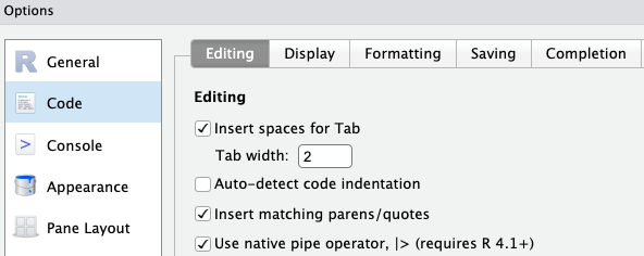
However, by default this (still) inserts an older pipe symbol, %>%. As long as you’ve loaded the tidyverse⁸, it would not really be a problem to just use %>% instead of |>. But it would be preferred to make RStudio insert the |> pipe symbol:

Click Tools > Global Options > Code tab on the right
Check the box “Use native pipe operator” as shown below
Click OK at the bottom of the options dialog box to apply the change and close the box.

8.7 Learn even more

The material in this page was adapted from this Carpentries lesson episode, which has a lot more content than we were able to cover today.

Regarding data wrangling specifically, here are two particularly useful additional skills to learn:

Pivoting/reshaping — moving between ‘wide’ and ‘long’ data formats with pivot_wider() and pivot_longer(). This is covered in episode 13 of the focal Carpentries lesson.
Joining/merging — combining multiple dataframes based on one or more shared columns. This can be done with dplyr’s join_*() functions – see for example this chapter in R for Data Science.

Footnotes

Or Click File => New file => R Script.↩︎
If not: run install.packages("tidyverse") now.↩︎
If not: run install.packages("gapminder") now.↩︎
The main difference is the nicer default printing behavior of tibbles: e.g. the data types of columns are shown, and only a limited number of rows are printed.↩︎
Using pipes is also faster and uses less computer memory.↩︎
Using the readxl package. This is installed as part of the tidyverse but is not a core tidyverse package and therefore needs to be loaded separately: library(readxl).↩︎
Recall that you can see where that is at the top of the Console tab, or by running getwd().↩︎
This symbol only works when you have one of the tidyverse packages loaded.↩︎

1 Introduction

1.1 What we’ll cover

1.2 Setting up

1.3 The dplyr package and the tidyverse

1.4 Loading the tidyverse

2 The gapminder dataset

3 arrange()

Challenge 1: arrange()

4 filter()

4.1 Filter based on one condition

4.2 Filter based on multiple conditions

5 The pipe (|>)

Challenge 2: Find the mistakes

Challenge 3: Find the extremes

6 mutate()

Challenge 4: Absolute GDP

7 summarize()

Challenge 5: Mean life expectancy

8 Bonus material for self-study

8.1 Writing and reading tabular data to and from files

Writing to files

Reading from files

8.2 rename() to change column names

8.3 select() to pick columns (variables)

8.4 Counting rows with count()

8.5 Function name conflicts

8.6 Using the pipe keyboard shortcut

8.7 Learn even more

Footnotes

2 The `gapminder` dataset

3 `arrange()`

Challenge 1: `arrange()`

4 `filter()`

5 The pipe (`|>`)

6 `mutate()`

7 `summarize()`

8.2 `rename()` to change column names

8.3 `select()` to pick columns (variables)

8.4 Counting rows with `count()`