Introduction to R and RStudio

Author

Software Carpentry / Horacio Lopez-Nicora

Published

August 18, 2025

1 Overview

1.1 This session

In this session, we will learn how to find your way around RStudio, how to interact with R, how to manage your R environment, and how to install packages. Our objectives include:

Describing the purpose and use of each pane in RStudio
Locating buttons and options in RStudio
Defining a variable/object
Assigning data to a variable/object
Managing a workspace in an interactive R session
Using mathematical and comparison operators
Calling functions
Managing packages
Getting help in R

By the end of this session, you will be well-equipped with the foundational skills needed to navigate RStudio and effectively interact with R.

1.2 The rest of today

We will begin with raw data, perform exploratory analyses, and learn how to plot results graphically. This example starts with a dataset from gapminder.org containing population information for many countries through time. Can you read the data into R? Can you plot the population for Senegal? Can you calculate the average income for countries on the continent of Asia? By the end of these lessons you will be able to do things like plot the populations for all of these countries in under a minute!

2 Why use R and R studio?

Science is a multi-step process: once you’ve designed an experiment and collected data, the real fun begins with analysis! In this lesson, we will teach you some of the fundamentals of the R language and share best practices for organizing code in scientific projects, which will make your life easier.

Though we could use a spreadsheet in Microsoft Excel or Google Sheets to analyze our data, these tools have limitations in terms of flexibility and accessibility. Moreover, they make it difficult to share the steps involved in exploring and modifying raw data, which is essential for conducting “reproducible” research.

Therefore, this lesson will guide you on how to start exploring your data using R. R is a program available for Windows, Mac, and Linux operating systems, and can be freely downloaded from the link provided above. To run R, all you need is the R program.

However, we will be running R inside a fancy editor (or “IDE”, Integrated Development Environment) called RStudio, which makes working with R much more pleasant!

Since R is open source, there are endlessly available free resource to learn how to do practically whatever you want on the internet.

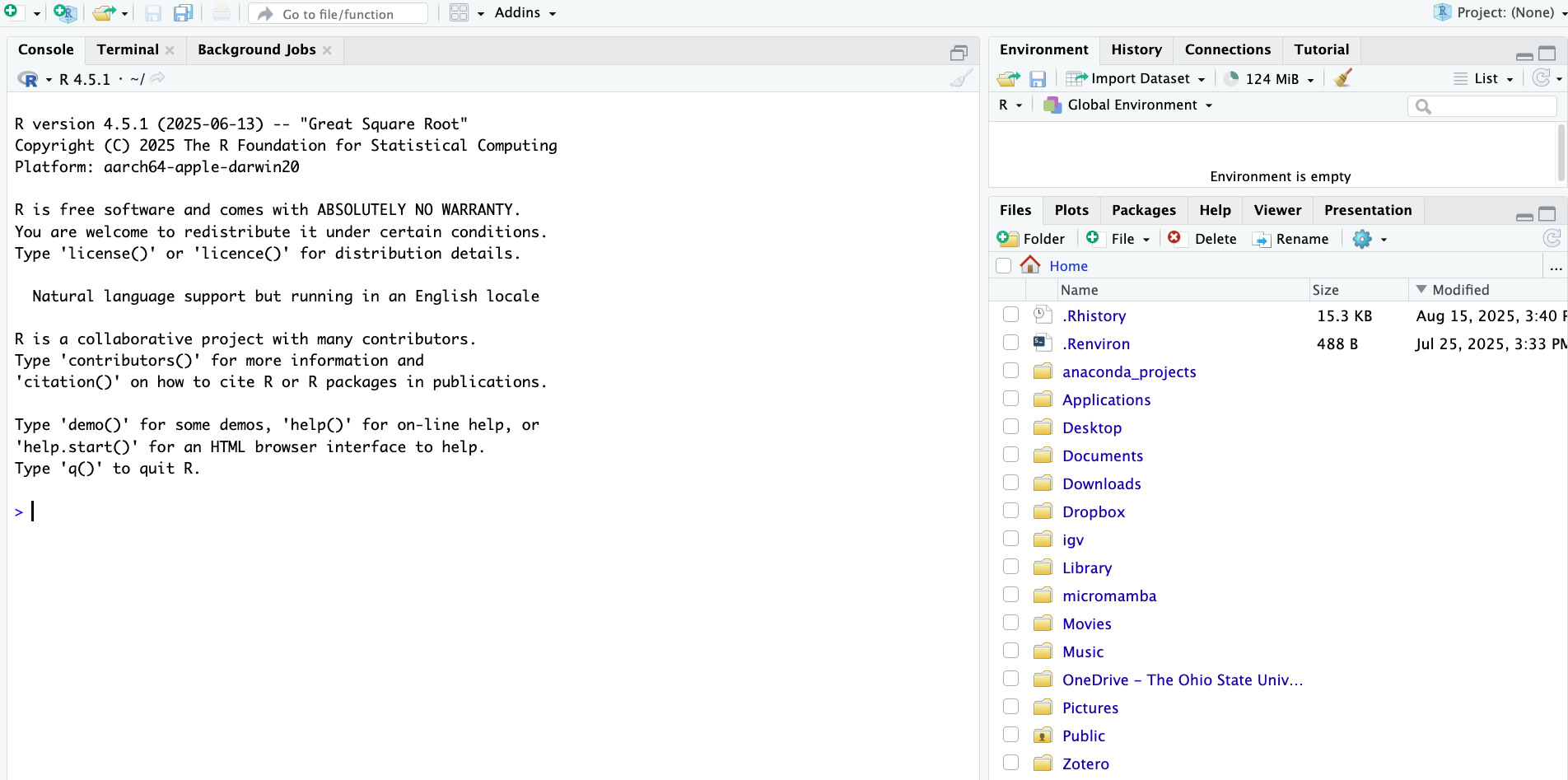
3 Orienting to RStudio (basic layout)

When you first open RStudio, you will be greeted by three panels:

Left: the default tab in this panel is your R “Console”, where you can type and execute R code (if you’ve previously used standalone R without RStudio, all that would be shown is this type of console).
Top right: the default tab in this panel this is your “Environment”, which shows you all the objects that are active in your R environment.
Bottom right: the default tab in this panel is “Files”, showing the files in your working directory (more about that next). There are also additional tabs to e.g. show plots, packages, and help, some of which we’ll see later today.

Click here for a useful RStudio cheatsheet

4 R as calculator

To get used to typing and executing R code, we’ll simply use R as a calculator – type 5 + 5 in the console and press Enter:

#Addition
5 + 5

[1] 10

R will print the result of the calculation, 10. The result is prefaced by [1], which is simply an index/count of outputs, because sometimes R can output hundreds of numbers or other elements.

More examples

# Subtraction
15 - 4

[1] 11

# Multiplication
6 * 8

[1] 48

# Division
40 / 5

[1] 8

# Exponents
3 ^ 4

[1] 81

# Square root (using exponent 0.5)
16 ^ 0.5

[1] 4

# Parentheses change order of operations
(5 + 3) * 2

[1] 16

# Without parentheses, multiplication happens first
5 + 3 * 2

[1] 11

# Multiple operations in one line
10 - 2 + 4 * 3

[1] 20

# Using ** as an alternative exponent operator
2 ** 5

[1] 32

Order of operations

When using R as a calculator, the order of operations is the same as you would have learned back in school. From highest to lowest precedence:

Parentheses: (, )
Exponents: ^ or **
Multiply: *
Divide: /
Add: +
Subtract: -

5 The R prompt

The > sign in your console is the R “prompt”. It indicates that R is ready for you to type something.

When you are not seeing the > prompt, R is either busy (because you asked it to do a longer-running computation) or waiting for you to complete an incomplete command.

If you notice that your prompt turned into a +, you typed an incomplete command – for example:

10 /

To get out of this situation, one option is to try and finish the command (in this case, by typing another number) — but here, let’s practice another option: aborting the command by pressing Esc.

6 R scripts

Once you open a file, a new RStudio panel will appear in the top-left, where you can view and edit text files, most commonly R scripts (.R). An R script is a text file that contains R code.

Create and open a new R script by clicking File (top menu bar) > New File > R Script.

Why use a script?

It’s a good idea to write and save most of our code in scripts, instead of directly in the R console. This helps us keep track of what we’ve been doing, especially in the longer run, and to re-run our code after modifying input data or one of the lines of code.

Sending code to the console

To send code from the editor to the console, where it will be executed by R, press Ctrl + Enter (or, on a Mac: Cmd + Enter) with the cursor anywhere in a line of code in the script.

Practice that after typing the following command in the script:

5 + 5

[1] 10

7 Adding comments to your code

You can use # signs to comment your code.

Anything to the right of a # is ignored by R, meaning it won’t be executed.
You can use # both at the start of a line (entire line is a comment) or anywhere in a line following code (rest of the line is a comment).
In your R script, comments are formatted differently so you can clearly distinguish them from code.

See the example below:

# This line is entirely ignored by R
10 / 5  # This line contains code but everythig after the '#' is ignored

[1] 2

8 Functions in R – and packages

To do almost anything in R, you will use “functions” (these are like commands).

You can recognize function calls by the parentheses, like in install.packages(). Inside those parentheses, you can provide arguments to a function.

For example, install.packages() is an important function you already used if you followed the setup instructions for this workshop: it will install an R package. R packages are basically add-ons or extensions to the functionality of the R language. Inside the parenthese of install.packages(), you should provide a package name as an argument, like install.packages("gapminder").

Another example of an R function is library(), which will access your “library” of installed packages to load a package. Every time you want to use a package in R, you need to load it, just like everytime you want to use MS Word on your computer, you need to open it.

Let’s see if you have the two packages that we will use today installed:

library(gapminder)
# (No output is expected if the package can be loaded)

# (Output like that shown below is expected if the package can be loaded:)
library(tidyverse)

── Attaching core tidyverse packages ──────────────────────── tidyverse 2.0.0 ──
✔ dplyr     1.1.4     ✔ readr     2.1.5
✔ forcats   1.0.0     ✔ stringr   1.5.1
✔ ggplot2   3.5.2     ✔ tibble    3.3.0
✔ lubridate 1.9.4     ✔ tidyr     1.3.1
✔ purrr     1.1.0     
── Conflicts ────────────────────────────────────────── tidyverse_conflicts() ──
✖ dplyr::filter() masks stats::filter()
✖ dplyr::lag()    masks stats::lag()
ℹ Use the conflicted package (<http://conflicted.r-lib.org/>) to force all conflicts to become errors

If you got an error when trying to load one or both of these packages, you’ll need to install those:

# ONLY run this if you got errors above:
install.packages("gapminder")
install.packages("tidyverse")

8.1 Some other R functions

Another important function is c(), which stands for combine or concatenate. With c(), you can create vectors that contain multiple elements, like multiple numbers. You’ll learn more about vectors in the next session, but here is a quick example:

c(10, 15)

[1] 10 15

Below are examples of some other R functions:


Function	Description
abs(x)	absolute value
sqrt(x)	square root
round(x, digits=n)	round(3.475, digits=2) is 3.48
log(x)	natural logarithm
log10(x)	common logarithm

9 Comparing things

In R, you can use comparison operators to compare numbers. For example:

# Greater than
8 > 3

[1] TRUE

# Less than
2 < 1

[1] FALSE

# Equal to
7 == 7

[1] TRUE

# Not equal to
10 != 5

[1] TRUE

# Greater than or equal to
6 >= 6

[1] TRUE

# Comparisons can be combined with arithmetic
(3 + 4) == 7

[1] TRUE

Here are the most common comparison operators in R:


Operator	Description	Example
>	Greater than	5 > 6 returns `FALSE`
<	Less than	5 < 6 returns `TRUE`
==	Equals to	10 == 10 returns `TRUE`
!=	Not equal to	10 != 10 returns `FALSE`
>=	Greater than or equal to	5 >= 6 returns `FALSE`
<=	Less than or equal to	6 <= 6 returns `TRUE`

10 R objects

10.1 Assigning stuff to objects

We can assign one or more values to a so-called “object” with the assignment operator <-. A few examples:

# Assign the value 250 the object 'length_cm'
length_cm <- 250

# Assign the value 2.54 to the object 'conversion'
conversion <- 2.54

To see the contents of an object, you can simply print its name:

length_cm

[1] 250

Importantly, you can use objects as if you had typed their values directly:

length_cm / conversion

[1] 98.4252

length_in <- length_cm / conversion
length_in

[1] 98.4252

10.2 Object names

Some pointers on object names:

Because R is case sensitive, length_inch is different from Length_Inch!
An object name cannot contain spaces — so for readability, you should separate words using:
- Underscores: length_inch (this is called “snake case”)
- Periods: wingspan.inch
- Capitalization: wingspanInch or WingspanInch (“camel case”)
You will make things easier for yourself by naming objects in a consistent way, for instance by always sticking to your favorite case style like “snake case.”
Object names can contain but cannot start with a number: x2 is valid but 2x is not.
Make object names descriptive yet not too long — this is not always easy!

11 R Help: `help()` and `?`

The help() function and ? help operator in R offer access to documentation pages for R functions, data sets, and other objects. They provide access to both packages in the standard R distribution and contributed packages.

For example:

?install.packages

The output should be shown in the Viewer tab of the bottom left RStudio panel, and look something like this:

12 Working directories

12.1 What is a directory and a working directory?

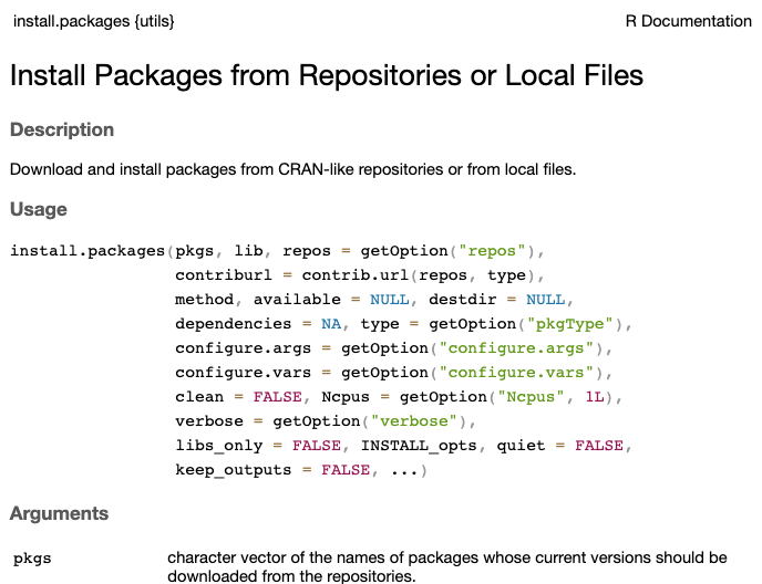
Understanding directories and your working directory is crucial when coding.

The word “directory” is just a synonym for a computer folder. These folders have specific physical locations on your computer, known as paths. Directories are organized hierarchically, and the overall structure of standard directories differs slightly across various operating systems, such as Mac, Windows, and Linux. By using Finder (Mac) or File Explorer (Windows), you can navigate to different locations on your computer, but you can also do so using R code.

Your working directory is exactly what it sounds like— it is the current location or path on your computer where you are actively working. This is important because, by default, your files will be read from, stored in, and saved to this location. Therefore, it is essential to know where your working directory is.

12.2 Find your working directory

We can figure out where our working directory is by typing the function getwd() into the console:

getwd()

[1] "/Users/lopez-nicora.1"

Directories are separated by / on Mac and by \ on Windows

Because I am using a Mac, directories in my path are separated by forward slashes /, while on Windows machines, they are separated by backslashes \.

That said, when you provide a path to R, like we’ll do below with setwd(), you can use forward slashes on all operating systems!

12.3 Set your working directory

If your working directory is not where you want to be, you can change it. We can do that using the function setwd():

setwd("/this/should/be/your/working-directory/path")

For example, I will change mine to:

setwd("~/Library/CloudStorage/OneDrive-TheOhioStateUniversity/Desktop/OSU - Soybean Pathology & Nematology/OSU - SOY PATH AND NEMA/YEAR - SEMESTER/2025/SUMMER 2025/EXTENSION AND OUTREACH/03_carpentries-aug-2025 - AUG_18_2025")

RStudio Projects

If you change your working dir in the R console, what is shown in the Files tab in the bottom-right does not automatically follow along. In that case, to show the files in your working dir in the Files tab, click the gear icon in that tab, and select Go To Working Directory.

However, there is a better way of dealing with working directories, which is to avoid using setwd() altogether and to use RStudio Projects instead.

To learn more about RStudio Projects, see this section in the free book R for Data Science.

1 Overview

1.1 This session

1.2 The rest of today

2 Why use R and R studio?

3 Orienting to RStudio (basic layout)

4 R as calculator

5 The R prompt

6 R scripts

Why use a script?

Sending code to the console

7 Adding comments to your code

8 Functions in R – and packages

8.1 Some other R functions

9 Comparing things

10 R objects

10.1 Assigning stuff to objects

10.2 Object names

11 R Help: help() and ?

12 Working directories

12.1 What is a directory and a working directory?

12.2 Find your working directory

12.3 Set your working directory

11 R Help: `help()` and `?`