Bonus material for self-study

Authors

Affiliation

Software Carpentry

Jelmer Poelstra

CFAES Bioinformatics Core, Ohio State University

Published

July 15, 2026

Modified

August 2, 2026

1 Bonus material for Session 2

1.1 Extracting elements from vectors

num_vec <- c(2, 6, 3, 41)

Extracting element from objects like vectors is often called indexing. In R, we can do this using “bracket notation” with square brackets [ ] — for example:

Get the second element with [2]¹:
```
num_vec[2]
```
```
[1] 6
```
Get the second through the fourth elements with [2:4]:
```
num_vec[2:4]
```
```
[1]  6  3 41
```

Challenge 3: Indexing

Given the fruits vector below, what does fruits[c(1, 3)] return?
```
fruits <- c("apple", "banana", "cherry", "pineapple")
```

This extracts the first and third elements of the fruits vector, returning:

fruits <- c("apple", "banana", "cherry", "pineapple")
fruits[c(1, 3)]

[1] "apple"  "cherry"

What do you expect fruits[5] will return?

A) "pineapple" B) An error C) "peach" D) Something else

The answer is: “D) Something else”.

fruits[5]

[1] NA

It returns NA, for missing data, because there is no fifth element in the vector.

Option C, an error, is a good guess as well, but R is designed to be forgiving in this case and returns NA instead of an error.

1.2 Changing vector elements using indexing

Above, we saw how you can extract elements of a vector using indexing. To change elements in a vector, simply use the bracket on the other side of the arrow – for example:

Change the first element to 30:
```
num_vec[1] <- 30
num_vec
```
```
[1] 30  6  3 41
```

Change the last element to 0:

num_vec[length(num_vec)] <- 0
num_vec

[1] 30  6  3  0

Change the second element to the mean value of the vector:

num_vec[2] <- mean(num_vec)
num_vec

[1] 30.00  9.75  3.00  0.00

1.3 The data frame data structure

One of R’s most powerful features is its built-in ability to deal with tabular data – i.e., data with rows and columns like you are familiar with from Excel spreadsheets and so on. In R, tabular data is stored in a data structure called “data frame”.

Let’s start by using the data.frame() function to make a data frame with information about 3 cats:

cats <- data.frame(
  name = c("Luna", "Thomas", "Daisy"),
  coat = c("calico", "black", "tabby"),
  weight = c(2.1, 5.0, 3.2)
)

cats

    name   coat weight
1   Luna calico    2.1
2 Thomas  black    5.0
3  Daisy  tabby    3.2

Above:

We created 3 vectors and pasted them side-by-side to create a data frame in which each vector constitutes a column.
We gave each vector a name (e.g., coat), and those names became the column names.
The resulting data frame has 3 rows (one for each cat) and 3 columns (each with a type of info about the cats, like coat color).

It is good practice to organize tabular data in the so-called “tidy” data format like above, where:

Each column contains a different “variable” (e.g. coat color, weight)
Each row contains a different “observation” (data on e.g. one cat/person/sample)

1.4 Extracting columns from a data frame

You can extract individual columns from a data frame using the $ operator:

cats$weight

[1] 2.1 5.0 3.2

cats$coat

[1] "calico" "black"  "tabby"

This kind of operation will return a vector — which can immediately be indexed as well:

cats$weight[2]

[1] 5

1.5 More on the `logical` data type

Let’s add a column to your cats data frame that indicates whether a cat likes string:

cats$likes_string <- c(1, 0, 1)
cats

    name   coat weight likes_string
1   Luna calico    2.1            1
2 Thomas  black    5.0            0
3  Daisy  tabby    3.2            1

So, likes_string is numeric, but the 1s and 0s are actually meant to represent true and false. Therefore, it would be better to use the logical data type here.

This can be achieved by converting this column with the as.logical() function. That will turn 0’s into FALSE and everything else, including 1, to TRUE:

as.logical(cats$likes_string)

[1]  TRUE FALSE  TRUE

To actually modify this column in the dataframe itself, you can assign the result of as.logical() back to the column:

cats$likes_string <- as.logical(cats$likes_string)
cats

    name   coat weight likes_string
1   Luna calico    2.1         TRUE
2 Thomas  black    5.0        FALSE
3  Daisy  tabby    3.2         TRUE

You might think that 1/0 is perhaps a handier coding than TRUE/FALSE, because it enables easy counting of the number of times something is true or false. But consider the following R behavior:

TRUE + TRUE

[1] 2

So, logicals can be used as if they were numbers, where FALSE represents 0 and TRUE represents 1 (!).

1.6 Missing values (`NA`)

R has a concept of missing data, which is important in statistical computing, because not all information/measurements are always available for each sample.

In R, missing values are coded as NA (like TRUE/FALSE, this is not a character string so it is not quoted):

# This vector will contain one missing value
vector_NA <- c(1, 3, NA, 7)
vector_NA

[1]  1  3 NA  7

Notably, many functions operating on vectors will return NA if any element in the vector is NA:

sum(vector_NA)

[1] NA

You can get around this is by setting na.rm = TRUE in such functions, for example:

sum(vector_NA, na.rm = TRUE)

[1] 11

1.7 Factors

Categorical data, like treatments in an experiment, can be stored as “factors” in R. Factors are useful for statistical analyses and for plotting, e.g. because they allow you to specify a custom order.

diet_vec <- c("high", "medium", "low", "low", "medium")
diet_vec

[1] "high"   "medium" "low"    "low"    "medium"

factor(diet_vec)

[1] high   medium low    low    medium
Levels: high low medium

In the example above, we turned a character vector into a factor. Its “levels” (low, medium, high) are sorted alphabetically by default, but we can manually specify an order that makes more sense:

diet_fct <- factor(diet_vec, levels = c("low", "medium", "high"))
diet_fct

[1] high   medium low    low    medium
Levels: low medium high

This ordering is automatically respected in plots and statistical analyses.

Oddly, factors are technically not a data type (Click to expand)

For most intents and purposes, it makes sense to think of factors as another data type, even though technically, they are a kind of data structure build on the integer data type:

typeof(diet_fct)

[1] "integer"

1.8 Learn more

To learn more about data types and data structures, see this episode from a separate Carpentries lesson.

Bonus Challenge

An important part of every data analysis is cleaning input data. Here, you will clean a cat data set that has an added observation with a problematic data entry.

Start by creating the new data frame:

cats_v2 <- data.frame(
  name = c("Luna", "Thomas", "Daisy", "Oliver"),
  coat = c("calico", "black", "tabby", "tabby"),
  weight = c(2.1, 5.0, 3.2, "2.3 or 2.4")
)

cats_v2

    name   coat     weight
1   Luna calico        2.1
2 Thomas  black          5
3  Daisy  tabby        3.2
4 Oliver  tabby 2.3 or 2.4

Then move on to the tasks below, filling in the blanks (______) and running the code:

The “weight” column has the incorrect data type ______. The correct data type is: ______.

The “weight” column has the incorrect data type character. The correct data type is: double/numeric.

Correct the 4^th weight with the mean of the two given values, then print the weight data frame to see the effect:

cats_v2$weight[4] <- 2.35
cats_v2$weight

[1] "2.1"  "5"    "3.2"  "2.35"

From the output of typeof(cats_v2$weight), we can see that the data type is still incorrect. Since the values are all quoted, the weight column is still a character vector, so we need to convert it to the correct data type.

Convert the weight column to the right data type:

cats_v2$weight <- as.double(cats_v2$weight)

Calculate the mean weight of the cats:

mean(cats_v2$weight)

[1] 3.1625

2 Bonus material for session 3

library(tidyverse)

── Attaching core tidyverse packages ──────────────────────── tidyverse 2.0.0 ──
✔ dplyr     1.2.1     ✔ readr     2.2.0
✔ forcats   1.0.1     ✔ stringr   1.6.0
✔ ggplot2   4.0.3     ✔ tibble    3.3.1
✔ lubridate 1.9.5     ✔ tidyr     1.3.2
✔ purrr     1.2.2     
── Conflicts ────────────────────────────────────────── tidyverse_conflicts() ──
✖ dplyr::filter() masks stats::filter()
✖ dplyr::lag()    masks stats::lag()
ℹ Use the conflicted package (<http://conflicted.r-lib.org/>) to force all conflicts to become errors

library(gapminder)

2.1 Writing and reading tabular data to and from files

When working with your own data in R, you’ll usually need to read data from files into your R environment, and conversely, to write data that is in your R environment to files.

While it’s possible to make R interact with Excel spreadsheet files², storing your data in plain-text files generally benefits reproducibility. Tabular plain text files can be stored using:

A Tab as the column delimiter (often called TSV files, and stored with a .tsv extension)
A comma as the column delimiter (often called CSV files, and stored with a .csv extension).

To practice writing and reading data to and from TSV files, the examples below use functions from the readr package. This package is part of the core tidyverse and therefore already loaded into your environment.

Writing to files

To write the gapminder data frame to a TSV file, use the write_tsv() function with argument x for the R object and argument file for the file path:

write_tsv(x = gapminder, file = "gapminder.tsv")

Because we simply provided a file name, the file will have been written in your R working directory³.

If you want to take a look at the file you just created, you can find it in RStudio’s Files tab and click on it, which will open it in the editor panel. Of course, you could also find it in your computer’s file browser and open it in different ways.

Want to write to a different folder on your computer? (Click to expand)

The file argument to write_tsv() takes a file path, meaning that you can specify any location on your computer for it, in addition to the file name.

For example, if you had a folder called results in your current working directory, you could save the file in there like so:

write_tsv(x = gapminder, file = "results/gapminder.tsv")

Note that a forward slash / as a folder delimiter will work regardless of your operating system (even though Windows natively delimits folder by a backslash \).

Finally, if you want to store the file in a totally different place than your working dir, it’s good to know that you can also use a so-called absolute (or “full”) path. For example:

write_tsv(x = gapminder, file = "/Users/poelstra.1/Desktop/gapminder.tsv")

Reading from files

To practice reading data from a file, use the read_tsv() function on the file you just created:

gapminder_reread <- read_tsv(file = "gapminder.tsv")

Rows: 1704 Columns: 6
── Column specification ────────────────────────────────────────────────────────
Delimiter: "\t"
chr (2): country, continent
dbl (4): year, lifeExp, pop, gdpPercap

ℹ Use `spec()` to retrieve the full column specification for this data.
ℹ Specify the column types or set `show_col_types = FALSE` to quiet this message.

Note that this function is rather chatty, telling you how many rows and columns it read, and what their data types are. Let’s check the resulting object:

gapminder_reread

# A tibble: 1,704 × 6
   country     continent  year lifeExp      pop gdpPercap
   <chr>       <chr>     <dbl>   <dbl>    <dbl>     <dbl>
 1 Afghanistan Asia       1952    28.8  8425333      779.
 2 Afghanistan Asia       1957    30.3  9240934      821.
 3 Afghanistan Asia       1962    32.0 10267083      853.
 4 Afghanistan Asia       1967    34.0 11537966      836.
 5 Afghanistan Asia       1972    36.1 13079460      740.
 6 Afghanistan Asia       1977    38.4 14880372      786.
 7 Afghanistan Asia       1982    39.9 12881816      978.
 8 Afghanistan Asia       1987    40.8 13867957      852.
 9 Afghanistan Asia       1992    41.7 16317921      649.
10 Afghanistan Asia       1997    41.8 22227415      635.
# ℹ 1,694 more rows

This looks good! Do note that the column’s data types are not identical to what they were (year and pop are saved as double rather than integer, and country and continent as character rather than factor). This is largely expected because that kind of metadata is not stored in a plain-text TSV, so read_tsv() will by default simply make best guesses as to the types.

Alternatively, you could tell read_tsv() what the column types should be, using the col_types argument (with abbreviations f for factor, i for integer, d for double — run ?read_tsv for more info):

read_tsv(file = "gapminder.tsv", col_types = "ffidi")

# A tibble: 1,704 × 6
   country     continent  year lifeExp      pop gdpPercap
   <fct>       <fct>     <int>   <dbl>    <int>     <dbl>
 1 Afghanistan Asia       1952    28.8  8425333      779.
 2 Afghanistan Asia       1957    30.3  9240934      821.
 3 Afghanistan Asia       1962    32.0 10267083      853.
 4 Afghanistan Asia       1967    34.0 11537966      836.
 5 Afghanistan Asia       1972    36.1 13079460      740.
 6 Afghanistan Asia       1977    38.4 14880372      786.
 7 Afghanistan Asia       1982    39.9 12881816      978.
 8 Afghanistan Asia       1987    40.8 13867957      852.
 9 Afghanistan Asia       1992    41.7 16317921      649.
10 Afghanistan Asia       1997    41.8 22227415      635.
# ℹ 1,694 more rows

To read and write CSV files instead, use read_csv() / write_csv() in the same way.

2.2 `rename()` to change column names

The rename() dplyr function is one of the package’s simplest, but it is very useful when you want to change column names.

The syntax to specify the new and old name within the function is new_name = old_name. For example, to rename the gdpPercap column:

rename(.data = gapminder, gdp_per_capita = gdpPercap)

# A tibble: 1,704 × 6
   country     continent  year lifeExp      pop gdp_per_capita
   <fct>       <fct>     <int>   <dbl>    <int>          <dbl>
 1 Afghanistan Asia       1952    28.8  8425333           779.
 2 Afghanistan Asia       1957    30.3  9240934           821.
 3 Afghanistan Asia       1962    32.0 10267083           853.
 4 Afghanistan Asia       1967    34.0 11537966           836.
 5 Afghanistan Asia       1972    36.1 13079460           740.
 6 Afghanistan Asia       1977    38.4 14880372           786.
 7 Afghanistan Asia       1982    39.9 12881816           978.
 8 Afghanistan Asia       1987    40.8 13867957           852.
 9 Afghanistan Asia       1992    41.7 16317921           649.
10 Afghanistan Asia       1997    41.8 22227415           635.
# ℹ 1,694 more rows

2.3 `select()` to pick columns (variables)

The select() dplyr function subsets a data frame by including/excluding certain columns. By default, it only includes the columns you specify:

gapminder |>
  select(year, country, pop)

# A tibble: 1,704 × 3
    year country          pop
   <int> <fct>          <int>
 1  1952 Afghanistan  8425333
 2  1957 Afghanistan  9240934
 3  1962 Afghanistan 10267083
 4  1967 Afghanistan 11537966
 5  1972 Afghanistan 13079460
 6  1977 Afghanistan 14880372
 7  1982 Afghanistan 12881816
 8  1987 Afghanistan 13867957
 9  1992 Afghanistan 16317921
10  1997 Afghanistan 22227415
# ℹ 1,694 more rows

The order of the columns in the output data frame is exactly as you list them in select(), and doesn’t need to be the same as in the input data frame. In other words, select() is also one way to reorder columns: in the example above, we made year appear before country.

You can also specify columns that should be excluded, by prefacing their name with a ! (or a -):

# This will include all columns _except_ continent:
gapminder |>
  select(!continent)

# A tibble: 1,704 × 5
   country      year lifeExp      pop gdpPercap
   <fct>       <int>   <dbl>    <int>     <dbl>
 1 Afghanistan  1952    28.8  8425333      779.
 2 Afghanistan  1957    30.3  9240934      821.
 3 Afghanistan  1962    32.0 10267083      853.
 4 Afghanistan  1967    34.0 11537966      836.
 5 Afghanistan  1972    36.1 13079460      740.
 6 Afghanistan  1977    38.4 14880372      786.
 7 Afghanistan  1982    39.9 12881816      978.
 8 Afghanistan  1987    40.8 13867957      852.
 9 Afghanistan  1992    41.7 16317921      649.
10 Afghanistan  1997    41.8 22227415      635.
# ℹ 1,694 more rows

There are also ways to e.g. select ranges of columns that are beyond the scope of this short workshop. Check the select() help by typing ?select to learn more.

2.4 Counting rows with `count()`

A common operation is simply counting the number of observations for each group. For instance, to check the number of countries included in the dataset for the year 2002, you can use the count() function. It takes the name of one or more columns to define the groups we are interested in, and can optionally sort the results in descending order with sort = TRUE:

gapminder |>
  filter(year == 2002) |>
  count(continent, sort = TRUE)

# A tibble: 5 × 2
  continent     n
  <fct>     <int>
1 Africa       52
2 Asia         33
3 Europe       30
4 Americas     25
5 Oceania       2

2.5 Function name conflicts

When you loaded the tidyverse, the output included a “Conflicts” section that may have seemed ominous:

── Conflicts ────────────────────────────────────────── tidyverse_conflicts() ──
✖ dplyr::filter() masks stats::filter()
✖ dplyr::lag()    masks stats::lag()
ℹ Use the conflicted package (<http://conflicted.r-lib.org/>) to force all conflicts to become errors

What this means is that two tidyverse functions, filter() and lag(), have the same names as two functions from the stats package that were already in your R environment.

Those stats package functions are part of what is often referred to as “base R”: core R functionality that is always available (loaded) when you start R.

Due to this function name conflict/collision, the filter() function from dplyr “masks” the filter() function from stats. Therefore, if you write a command with filter(), it will use the dplyr function and not the stats function.

You can use a “masked” function, by prefacing it with its package name as follows: stats::filter().

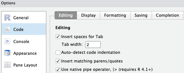
2.6 Using the pipe keyboard shortcut

The following RStudio keyboard shortcut will insert a pipe symbol: Ctrl/Cmd + Shift + M.

However, by default this (still) inserts an older pipe symbol, %>%. As long as you’ve loaded the tidyverse⁴, it would not really be a problem to just use %>% instead of |>. But it would be preferred to make RStudio insert the |> pipe symbol:

Click Tools > Global Options > Code tab on the right
Check the box “Use native pipe operator” as shown below
Click OK at the bottom of the options dialog box to apply the change and close the box.

2.7 Learn even more

The material in this page was adapted from this Carpentries lesson episode, which has a lot more content than we were able to cover today.

Regarding data wrangling specifically, here are two particularly useful additional skills to learn:

Pivoting/reshaping — moving between ‘wide’ and ‘long’ data formats with pivot_wider() and pivot_longer(). This is covered in episode 13 of the focal Carpentries lesson.
Joining/merging — combining multiple dataframes based on one or more shared columns. This can be done with dplyr’s join_*() functions – see for example this chapter in R for Data Science.

Footnotes

R uses 1-based indexing, which means it starts counting at 1 like humans do. Index 2 therefore simply corresponds to the second element. Python and several other languages use 0-based indexing, which starts counting at 0 such that the second element corresponds to index 1.↩︎
Using the readxl package. This is installed as part of the tidyverse but is not a core tidyverse package and therefore needs to be loaded separately: library(readxl).↩︎
Recall that you can see where that is at the top of the Console tab, or by running getwd().↩︎
This symbol only works when you have one of the tidyverse packages loaded.↩︎

1 Bonus material for Session 2

1.1 Extracting elements from vectors

Challenge 3: Indexing

1.2 Changing vector elements using indexing

1.3 The data frame data structure

1.4 Extracting columns from a data frame

1.5 More on the logical data type

1.6 Missing values (NA)

1.7 Factors

1.8 Learn more

Bonus Challenge

2 Bonus material for session 3

2.1 Writing and reading tabular data to and from files

Writing to files

Reading from files

2.2 rename() to change column names

2.3 select() to pick columns (variables)

2.4 Counting rows with count()

2.5 Function name conflicts

2.6 Using the pipe keyboard shortcut

2.7 Learn even more

Footnotes

1.5 More on the `logical` data type

1.6 Missing values (`NA`)

2.2 `rename()` to change column names

2.3 `select()` to pick columns (variables)

2.4 Counting rows with `count()`